Raster Ingestion Pipeline

fused.h3.run_ingest_raster_to_h3() converts large rasters to H3 in one call. Besides assigning pixels to hexes, it aggregates the values in each hex with the metric you choose (avg, cnt, ...) and writes overview files at coarser resolutions for fast zoomed-out views. Read the result with read_h3_dataset().

Use it for single-band rasters, especially categorical or high-resolution ones such as the Cropland Data Layer (CDL). It does more for you than partition, index & query, but it reads single-band rasters only and has no date or scenario folders to filter on. For points, vectors, tables or multi-dimensional data, use partition, index & query. See Choose your path.

Explore pre-ingested datasets in Canvas →

Basic Example

@fused.udf
def udf():
    input_path = "s3://fused-asset/data/nyc_dem.tif"
    output_path = "s3://fused-users/fused/joris/nyc_dem_h3/"  # <-- update this path

    result_extract, result_partition = fused.h3.run_ingest_raster_to_h3(
        input_path,
        output_path,
        metrics=["avg"],
    )

    # verify ingestion succeeded
    if not result_extract.all_succeeded():
        print(result_extract.errors())
    if result_partition is not None and not result_partition.all_succeeded():
        print(result_partition.errors())

This produces H3 hexagon data like:

hex	data_avg	source_url	res
617733120275513343	9.59	s3://fused-asset/data/nyc_dem.tif	9
617733120275775487	-2.473	s3://fused-asset/data/nyc_dem.tif	9
617733120276037631	14.484	s3://fused-asset/data/nyc_dem.tif	9
617733120276299775	-2.473	s3://fused-asset/data/nyc_dem.tif	9

Open in HyParquet to explore the full file.

Required parameters:

input_path: Raster file path(s) on S3 (TIFF or any GDAL-readable format)
output_path: Writable S3 location for output
metrics: Aggregation method per H3 cell ("avg", "sum", "cnt", "min", "max", "stddev")

How It Works

The function runs multiple UDFs in parallel under the hood. The orchestrating UDF doesn't need much resources, but can exceed the 2-min realtime limit. For larger data, use a batch instance:

@fused.udf(engine="small")
def udf():
    input_path = "s3://fused-asset/data/nyc_dem.tif"
    ...

Output Structure

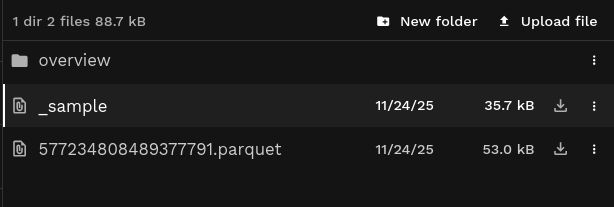
The ingestion creates:

Parquet data files (e.g., 577234808489377791.parquet) - each row is an H3 cell with hex ID + computed values
_sample metadata file - chunk/file bounding boxes for fast spatial queries
/overview/ directory - pre-aggregated files at lower resolutions (hex3.parquet, hex4.parquet, etc.)

Files created by the ingestion process

Overview file (/overview/hex7.parquet) — example rows (hex ID + aggregated value):

hex	data_avg
872830828ffffff	12.4
87283082effffff	8.2
87283082dffffff	15.1
87283082bffffff	3.7
872830829ffffff	22.0

Open in HyParquet to explore the full file.

Metrics

Choose metrics based on your raster data type:

Metric	Use Case	Output Columns
`"cnt"`	Categorical data (land use, crop types)	`data`, `cnt`, `cnt_total`
`"avg"`	Continuous averages (temperature, elevation, density)	`data_avg`
`"sum"`	Totals (population counts)	`data_sum`
`"min"`, `"max"`, `"stddev"`	Additional statistics	`data_min`, `data_max`, `data_stddev`

note

"cnt" cannot be combined with other metrics. Other metrics can be combined: metrics=["avg", "min", "max"]

Counting (categorical data)

For discrete/categorical rasters like land use, "cnt" counts occurrences per category:

CDL Example

@fused.udf
def udf(
    bounds: fused.types.Bounds = [-73.983, 40.763, -73.969, 40.773],
    res: int = None,
):
    # Cropland Data Layer ingested with "cnt" metric
    path = "s3://fused-asset/hex/cdls_v8/year=2024/"
    utils = fused.load("https://github.com/fusedio/udfs/tree/9780aef/community/joris/Read_H3_dataset")
    df = utils.read_h3_dataset(path, bounds, res=res)
    return df

                  hex  data  cnt  cnt_total
626740321835323391   122   12         14
626740321835323391   123    1         14
626740321835323391   121    1         14

Each H3 cell can have multiple rows (one per category).

Aggregating (continuous data)

For continuous rasters, aggregation produces one value per H3 cell:

DEM Example

@fused.udf
def udf(
    bounds: fused.types.Bounds = [-73.983, 40.763, -73.969, 40.773],
    res: int = None,
):
    path = "s3://fused-asset/hex/nyc_dem/"
    utils = fused.load("https://github.com/fusedio/udfs/tree/9780aef/community/joris/Read_H3_dataset")
    df = utils.read_h3_dataset(path, bounds, res=res)
    return df

                  hex   data_avg
0  617733122581069823  78.822576
1  617733122610954239  78.225562

Configuration

Data Resolution (`res`)

By default, resolution is inferred from raster pixel size. Override with res parameter.

See Resolution Guide for the full resolution table.

Partitioning (`file_res`, `chunk_res`)

Data is spatially partitioned using H3:

Parameter	Purpose	Default
`file_res`	Split into multiple files	Inferred (~100MB-1GB per file)
`chunk_res`	Row groups within files	Inferred (~1M rows per chunk)
`max_rows_per_chunk`	Alternative to `chunk_res`	-

Special case: file_res=-1 creates a single output file for smaller datasets.

Example

For data resolution 10: default file_res=0 (max 122 files globally) and chunk_res=3 (max 343 row groups per file, ~820k rows each assuming full coverage).

Overview Resolutions (`overview_res`)

Overviews are pre-aggregated files for fast zoomed-out views. Default: resolutions 3-7.

# doctest: skip
result_extract, result_partition = fused.h3.run_ingest_raster_to_h3(
    input_path,
    output_path,
    metrics=["avg"],
    overview_res=[7,6,5,4,3],  # Custom overview resolutions
)

Overview files are also chunked. Default chunk resolution is overview_res - 5. Override with overview_chunk_res or max_rows_per_chunk.

Multiple Files

Single file:

input_path = "s3://fused-asset/data/nyc_dem.tif"

Directory:

input_path = fused.api.list("s3://copernicus-dem-90m/")

Multiple paths:

input_path = [
    "s3://copernicus-dem-90m/.../file1.tif",
    "s3://copernicus-dem-90m/.../file2.tif",
]

Ingesting more than 20 files

When ingesting a single or up to 20 files, each file is processed in multiple chunks in the first "extract" step (number of chunks depending on target_chunk_size argument). But when processing more than 20 files, each file is processed as a single chunk by default (fetching the metadata of each input file to determine the chunking can take a lot of time if there are many input files). This might make the "extract" step require more memory. You can still override this default by specifying a specific target_chunk_size value.

info

Ingestion works with any hosted raster data - your files don't need to be on Fused's S3.

Execution Control

The ingestion runs these steps in parallel via .map():

extract: Assign pixel values to H3 cells
partition: Combine chunks per file, create metadata
overview: Create aggregated overview files

Override execution with:

engine: Specify execution engine (e.g., "small", "medium", "c2-standard-4"). Use extract_engine, partition_engine and overview_engine to specify the execution engine for only a single step.
extract_max_workers, partition_max_workers, overview_max_workers: Control parallelism for each step individually (there is no single generic max_workers or worker_concurrency argument)

Running on GCP

@fused.udf(engine="c2-standard-4")  # Orchestrator
def udf():
    result_extract, result_partition = fused.h3.run_ingest_raster_to_h3(
        input_path,
        output_path,
        metrics=["avg"],
        engine="c2-standard-60",  # Compute workers
    )

Reading Ingested Data

Use read_h3_dataset to automatically select data vs overview files based on viewport. The following example reads a public, pre-ingested copy of the NYC DEM dataset from the Basic Example above:

Open this UDF in Canvas → · Categorical (crop data) version →

@fused.udf
def udf(
    bounds: fused.types.Bounds = [-74.556, 40.400, -73.374, 41.029],
    res: int = None,
):
    path = "s3://fused-asset/hex/nyc_dem/"
    utils = fused.load("https://github.com/fusedio/udfs/tree/9780aef/community/joris/Read_H3_dataset/")
    df = utils.read_h3_dataset(path, bounds, res=res)
    return df

Visualizing Ingested Data

In Canvas, the UDF's output feeds a map widget:

To render the hexagons on a standalone map instead, use map_utils.deckgl_layers:

Standalone map code

@fused.udf
def udf(
    bounds: fused.types.Bounds = [-74.556, 40.400, -73.374, 41.029],
    res: int = 9,
):
    path = "s3://fused-asset/hex/nyc_dem/"
    utils = fused.load("https://github.com/fusedio/udfs/tree/9780aef/community/joris/Read_H3_dataset/")
    df = utils.read_h3_dataset(path, bounds, res=res)

    map_utils = fused.load("https://github.com/fusedio/udfs/tree/3ada22d/community/milind/map_utils")
    layers = [
        {
            "type": "hex",
            "data": df,
            "name": "NYC DEM H3 Hexagons",
            "config": {
                "style": {
                    "fillColor": {
                        "type": "continuous",
                        "attr": "data_avg",
                        "domain": [0, 400],
                        "steps": 20,
                        "palette": "BrwnYl",
                    },
                    "filled": True,
                    "extruded": False,
                    "stroked": False,
                    "opacity": 0.7,
                }
            },
        },
    ]
    return map_utils.deckgl_layers(layers=layers, basemap="dark")

For more on standalone maps, see Standalone Maps. For Workbench styling, see H3 Visualization.

Basic Example​

How It Works​

Output Structure​

Metrics​

Counting (categorical data)​

Aggregating (continuous data)​

Configuration​

Data Resolution (res)​

Partitioning (file_res, chunk_res)​

Overview Resolutions (overview_res)​

Multiple Files​

Execution Control​

Running on GCP​

Reading Ingested Data​

Visualizing Ingested Data​