Seismic Hazard Mapping

Cross-reference earthquake hazard with building density over Italy to find where the most buildings sit in the highest-risk zones.

Try the full canvas

Open the live canvas: Seismic Hazard Mapping

The problem

Italy sits at the collision of the African and Eurasian tectonic plates. Cities like L'Aquila and Amatrice have suffered devastating earthquakes in living memory. The goal: find where the highest concentration of buildings overlaps with the highest seismic hazard.

That requires joining two datasets that have nothing in common structurally — a raster and a vector — from two different organizations. H3 makes it trivial.

Data sources

• Seismic hazard — GEM Foundation OpenQuake Global Seismic Hazard Map (GSHM 2023). Each pixel is a Peak Ground Acceleration (PGA) value for a 1-in-475-year event.
• Buildings — Overture Maps building footprints for Italy, as pre-partitioned GeoParquet files.

Canvas overview

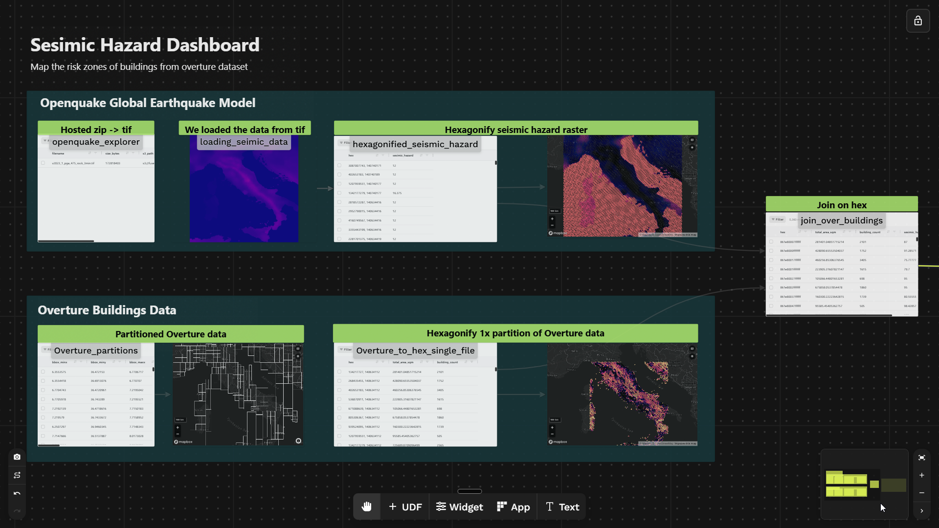
Step	UDF	What it does
1	openquake_explorer	Downloads the OpenQuake GeoTIFF and saves it to S3 once
2	loading_seismic_data	Reads the TIF for a given bounding box, returns a pixel array
3	hexagonified_seismic_hazard	Converts raster pixels → H3 hexagons, averaging hazard per cell
4	Overture_partitions	Shows Overture partition footprints across Italy
5	Overture_to_hex_single_file	Aggregates building area per H3 hex via DuckDB spatial SQL
6	join_over_buildings	Inner-joins both hex tables on H3 cell ID
7	Widget	Scatter chart + KPI tiles + map

1. Ingest the seismic GeoTIFF

The OpenQuake dataset is distributed as a ZIP containing a GeoTIFF. Rather than downloading it on every run, this UDF fetches it once and writes it to S3. Subsequent UDFs read from S3 directly.

View openquake_explorer code

@fused.udf
def udf(save_to_s3: bool = True):
    import pandas as pd
    import requests
    import io
    import zipfile

    url = "https://cloud.openquake.org/public.php/dav/files/6SnFk2f92JEr76H"

    @fused.cache  # <-- fetch once, re-use on subsequent runs
    def fetch_zip(url):
        response = requests.get(url, timeout=60)
        response.raise_for_status()
        return response.content

    content = fetch_zip(url)
    zf = zipfile.ZipFile(io.BytesIO(content))

    tif_name = "v2023_1_pga_475_rock_3min.tif"
    s3_path = f"s3://fused-asset/demos/seismic_data/{tif_name}"

    print(f"Extracting {tif_name} from ZIP...")
    tif_bytes = zf.read(tif_name)
    print(f"Extracted {len(tif_bytes):,} bytes")

    if save_to_s3:
        import s3fs
        fs = s3fs.S3FileSystem()
        with fs.open(s3_path, "wb") as f:
            f.write(tif_bytes)
        print(f"Saved to {s3_path}")

    return pd.DataFrame([{
        "filename": tif_name,
        "size_bytes": len(tif_bytes),
        "s3_path": s3_path,
        "status": "saved" if save_to_s3 else "dry_run"
    }])

tip

@fused.cache means the network request only runs once. See efficient caching.

2. Load the seismic raster

Reads the GeoTIFF from S3 clipped to a bounding box and returns a 2D NumPy array of PGA values. This array feeds directly into step 3, which converts it to H3 hexagons.

View loading_seismic_data code

@fused.udf
def udf(
    bounds: fused.types.Bounds = [6.6272, 36.6197, 18.4802, 47.0921],
    chip_len: int = 512
):
    path: str = 's3://fused-asset/demos/seismic_data/v2023_1_pga_475_rock_3min.tif'
    common = fused.load('https://github.com/fusedio/udfs/tree/6750f1f/public/common/')
    arr = common.read_tiff_safe(bounds, path, chip_len, max_pixel=10 ** 8)

    print(arr)
    return arr

3. Raster → H3 hexagons

arr_to_h3 samples each pixel's coordinate, assigns it to an H3 cell, and aggregates all pixels in the same cell into a mean hazard score. A GeoTIFF becomes a flat table: one row per hex, one hazard column.

@fused.udf
def udf(
    bounds: fused.types.Bounds = [6.6272, 36.6197, 18.4802, 47.0921],
    chip_len: int = 512,
    h3_res: int = 6
):
    import numpy as np
    common = fused.load('https://github.com/fusedio/udfs/tree/5610abb/public/common/')
    parent_udf = fused.load('loading_seimic_data')

    arr = parent_udf(bounds=bounds, chip_len=chip_len)
    if arr.ndim == 3:
        arr = arr[0]

    df = common.arr_to_h3(arr, bounds, res=h3_res)  # <-- raster pixels → H3 hexagons

    df["sesimic_hazard"] = df["agg_data"].apply(lambda x: float(np.mean(x)))  # <-- mean PGA per cell
    return df[["hex", "sesimic_hazard"]]

Output (30,031 hex cells for Italy at resolution 6):

hex	sesimic_hazard
604474434765455359	12.000
604474509390512127	12.000
604474458656210943	12.000
604474458790428671	16.375
604020220230631423	12.000

H3 resolution

Resolution 6 cells are ~36 km² — good for a country-scale overview. Resolution 7 (~5 km²) gives finer detail. See the resolution guide.

4. Explore Overture partitions

Overture building data is split into geographic partitions to keep file sizes manageable. Before reading buildings, you need to know which partition file covers your AOI. The interactive map below shows all partition boundaries across Italy — hover to see the file_id and pick the right file for step 5.

View Overture_partitions widget JSON

{
  "type": "fused-map",
  "props": {
    "basemap": "mapbox://styles/mapbox/dark-v11",
    "centerLng": 12.5,
    "centerLat": 42,
    "zoom": 5,
    "showControls": true,
    "showScale": true,
    "showBasemapSwitcher": true,
    "showLegend": false,
    "showLayerPanel": true,
    "autoSend": false,
    "autoSendDebounceMs": 600,
    "layers": [
      {
        "id": "partitions-layer",
        "name": "Overture Partitions",
        "type": "deck-geojson",
        "visible": true,
        "sql": "SELECT file_id, ST_AsGeoJSON(geometry) as geometry FROM {{Overture_partitions}}",
        "geometryColumn": "geometry",
        "tooltip": ["file_id"],
        "style": {
          "opacity": 0.8,
          "lineColor": [250, 250, 250],
          "lineWidth": 1,
          "fillColor": [0, 0, 0, 0]
        }
      }
    ]
  }
}

5. Buildings → H3 with DuckDB

Each Overture partition contains tens of thousands of building polygons. This UDF reads one partition and uses DuckDB's spatial extensions to compute centroids, assign H3 cells, and aggregate total area and building count — all in a single SQL pass. The result has the same shape as the seismic layer from step 3: one row per H3 cell, ready to join.

@fused.udf
def udf(
    path: str = "s3://fused-asset/overture/2026-03-18.0/theme=buildings/type=building/part=2/36.parquet",
    res: int = 6
):
    import geopandas as gpd

    common = fused.load("https://github.com/fusedio/udfs/tree/4dde28e/public/common/")
    con = common.duckdb_connect()
    gdf = con.sql(f"""
        SELECT
            h3_latlng_to_cell(ST_Y(ST_Centroid(geometry::GEOMETRY)), ST_X(ST_Centroid(geometry::GEOMETRY)), {res}) AS hex,
            sum(ST_Area_Spheroid(geometry::GEOMETRY)) as total_area_sqm,
            count(1) as building_count
        FROM read_parquet('{path}')
        group by 1
        order by 1
    """).df()
    return gdf.reset_index(drop=True)

6. Join on H3

The outputs of hexagonified_seismic_hazard and Overture_to_hex_single_file UDF both share a hex column at the same resolution. That's the key insight: by expressing both datasets on the same H3 grid, joining a raster and a vector becomes a standard table join. The result has one row per hex cell with hazard score and building statistics side by side — ready for analysis.

View join_over_buildings code

@fused.udf
def udf(
    path: str = "s3://fused-asset/overture/2026-03-18.0/theme=buildings/type=building/part=2/36.parquet",
    res: int = 6,
    bounds: fused.types.Bounds = [6.6272, 36.6197, 18.4802, 47.0921],
    chip_len: int = 512,
    h3_res: int = 6,
):
    import pandas as pd

    overture_udf = fused.load("Overture_to_hex_single_file")
    df_buildings = overture_udf(path=path, res=res)

    seismic_udf = fused.load("hexagonified_seismic_hazard")
    df_seismic = seismic_udf(bounds=bounds, chip_len=chip_len, h3_res=h3_res)

    # normalize to lowercase hex string (H3 canonical format) before joining
    df_buildings["hex"] = df_buildings["hex"].apply(lambda x: format(int(x), 'x'))
    df_seismic["hex"] = df_seismic["hex"].apply(lambda x: format(int(x), 'x'))

    return pd.merge(df_buildings, df_seismic, on="hex", how="inner")  # <-- join on H3 cell

A seismic hazard raster and building vector polygons — two completely different formats from two different organizations — unified with JOIN ON hex. Read more in joining H3 datasets.

7. Dashboard

The widget uses {{join_over_buildings}} to query the upstream UDF output directly. The scatter chart plots each hex cell as a point (x = hazard score, y = building count), colored by risk category. The map layer filters to only hexes above both thresholds, making the high-risk zones immediately visible. KPI tiles show aggregate counts across the filtered set.

View widget JSON

{
  "type": "div",
  "props": {
    "style": "display: flex; flex-direction: column; gap: 10px; padding: 14px; background: #1a1c1f; height: 100%; font-family: sans-serif; box-sizing: border-box;"
  },
  "children": [
    {
      "type": "div",
      "props": {
        "style": "display: flex; flex-direction: row; align-items: baseline; gap: 12px; flex: initial;"
      },
      "children": [
        {
          "type": "text",
          "props": {
            "content": "Seismic Hazard & Building Risk Dashboard",
            "variant": "h3",
            "style": "color: #f1f5f9; margin: 0; flex: initial;"
          }
        },
        {
          "type": "text",
          "props": {
            "content": "Hazard score vs. building count per H3 hex (res 6)",
            "variant": "muted",
            "style": "color: #94a3b8; font-size: 12px; flex: initial;"
          }
        }
      ]
    },
    {
      "type": "div",
      "props": {
        "style": "display: flex; flex-direction: row; gap: 10px; flex: initial;"
      },
      "children": [
        {
          "type": "big-number",
          "props": {
            "label": "High-Risk Zones",
            "sql": "SELECT COUNT(*) FROM {{join_over_buildings}} WHERE sesimic_hazard > 70 AND building_count > 1000",
            "style": "flex: 1; background: #212326; border-radius: 8px; padding: 8px 14px; border: 1px solid #E8FF59; color: #E8FF59;"
          }
        },
        {
          "type": "big-number",
          "props": {
            "label": "Avg Hazard Score",
            "sql": "SELECT ROUND(AVG(sesimic_hazard), 1) FROM {{join_over_buildings}} WHERE sesimic_hazard > 70 AND building_count > 1000",
            "style": "flex: 1; background: #212326; border-radius: 8px; padding: 8px 14px; border: 1px solid #E8FF59; color: #E8FF59;"
          }
        },
        {
          "type": "big-number",
          "props": {
            "label": "Buildings at Risk",
            "sql": "SELECT SUM(building_count) FROM {{join_over_buildings}} WHERE sesimic_hazard > 70 AND building_count > 1000",
            "style": "flex: 1; background: #212326; border-radius: 8px; padding: 8px 14px; border: 1px solid #E8FF59; color: #E8FF59;"
          }
        }
      ]
    },
    {
      "type": "div",
      "props": {
        "style": "display: flex; flex-direction: row; gap: 10px; flex: 1; min-height: 0;"
      },
      "children": [
        {
          "type": "fused-map",
          "props": {
            "basemap": "mapbox://styles/mapbox/dark-v11",
            "centerLng": 12.5,
            "centerLat": 42,
            "zoom": 5,
            "showControls": true,
            "showScale": false,
            "showBasemapSwitcher": true,
            "showLegend": true,
            "showLayerPanel": false,
            "autoSend": false,
            "autoSendDebounceMs": 600,
            "style": "flex: 1; border-radius: 10px; overflow: hidden; min-height: 0;",
            "layers": [
              {
                "id": "high-risk-h3",
                "name": "High-Risk Zones",
                "type": "h3",
                "visible": true,
                "sql": "SELECT hex, sesimic_hazard, building_count FROM {{join_over_buildings}} WHERE sesimic_hazard > 70 AND building_count > 1000",
                "h3Column": "hex",
                "tooltip": ["hex", "sesimic_hazard", "building_count"],
                "legend": { "title": "Seismic Hazard Score" },
                "style": {
                  "fillColor": {
                    "type": "continuous",
                    "attr": "sesimic_hazard",
                    "domain": [70, 100],
                    "colors": ["#fde68a", "#f97316", "#dc2626", "#7f1d1d"]
                  },
                  "opacity": 0.85,
                  "coverage": 0.9,
                  "extruded": false
                }
              }
            ]
          }
        },
        {
          "type": "scatter-chart",
          "props": {
            "title": "Seismic Hazard vs. Number of Buildings",
            "sql": "SELECT sesimic_hazard AS x, building_count AS y, CASE WHEN sesimic_hazard > 70 AND building_count > 1000 THEN 'High Risk' ELSE 'Lower Risk' END AS series FROM {{join_over_buildings}}",
            "pointColor": "#E8FF59",
            "pointOpacity": 0.75,
            "defaultPointSize": 5,
            "pointStrokeWidth": 0.35,
            "pointStrokeColor": "#1a1c1f",
            "minBubbleSize": 10,
            "maxBubbleSize": 140,
            "showGrid": true,
            "showLegend": true,
            "xAxisFontSize": 11,
            "yAxisFontSize": 11,
            "animationMs": 300,
            "style": "flex: 1; min-width: 260px; background: #212326; border-radius: 10px; padding: 10px; min-height: 0; overflow: hidden;"
          }
        }
      ]
    }
  ]
}

Styling the map

Customize colors, opacity, and coverage in the Visualization tab. You can also use the AI-driven widget to describe style changes in plain language and have them applied instantly.

Next steps

• Swap the AOI — replace the Italy bounds with Turkey, Japan, or the US West Coast
• Add vulnerability — join a third dataset (e.g. building age from Overture) to weight exposure by structural fragility
• Run at scale — use my_udf.map() to process all Overture partitions in parallel

Further reading:

• Converting to H3
• Resolution guide
• Geospatial ingestion