Converting Data to H3

This page covers different methods to convert your data into H3 hexagons.

---

File to H3

Turning a single small dataset into a grid of H3 hexagons.

Point Count to Hex

The following example uses a simple CSV of 311 calls in the New York City area, showing a heatmap of calls per hex 9 cell

Code

@fused.udf
def udf(
    res: int = 9
):
    noise_311_link = "https://gist.githubusercontent.com/kashuk/670a350ea1f9fc543c3f6916ab392f62/raw/4c5ced45cc94d5b00e3699dd211ad7125ee6c4d3/NYC311_noise.csv"
    # Load common utilities (includes duckdb helper)
    common = fused.load("https://github.com/fusedio/udfs/tree/b7637ee/public/common/")
    con = common.duckdb_connect()

    # Keep latitude and longitude (averaged per hex) alongside the hex count
    df = con.execute(
        """
        SELECT
          h3_latlng_to_cell(lat, lng, ?) AS hex,
          COUNT(*) AS cnt,
          AVG(lat) AS lat,
          AVG(lng) AS lng
        FROM read_csv_auto(?)
        WHERE lat IS NOT NULL AND lng IS NOT NULL
        GROUP BY 1
        """,
        [res, noise_311_link],
    ).df()

    # Debugging: print the resulting DataFrame schema
    print(df.T)

    return df

Requirements

• Small single (< 100MB) file (GeoJSON, CSV, Parquet, etc.). In example:

lat,lng
40.7128,-74.0060
40.7128,-74.0060

• Hexagon resolution (10, 11, 12, etc.). In this example:

res: int = 9

• Field to hexagonify & Aggregation function (max 'population', avg 'income', mean 'elevation', etc.). In this example simply counting the number of calls per hex:

# Keep latitude and longitude (averaged per hex) alongside the hex count
df = con.execute(
    """
    SELECT
        h3_latlng_to_cell(lat, lng, ?) AS hex,
        COUNT(*) AS cnt,
        AVG(lat) AS lat,
        AVG(lng) AS lng
    FROM read_csv_auto(?)
    WHERE lat IS NOT NULL AND lng IS NOT NULL
    GROUP BY 1
    """,
    [res, noise_311_link],
).df()

---

Dynamic Tile to H3

Dynamically tile data into H3 hexagons in a given viewport. Hex resolution is calculated based on the bounds of the viewport.

Set your UDF to Tile UDF Mode

The examples in this section all use Tile UDF Mode to dynamically compute H3 based on the viewport bounds.

Polygon to Hex

The following example uses a simplified Census Block Group dataset of the state of California, showing a heatmap of the population density per hex 9 cell:

Link to UDF in Fused Catalog

Code

@fused.udf
def udf(
    bounds: fused.types.Bounds = [-125.0, 24.0, -66.9, 49.0],
    min_hex_cell_res: int= 11, # Increase this if working with high res local data
    max_hex_cell_res: int= 4,
):
    import pandas as pd
    import geopandas as gpd
    
    common = fused.load("https://github.com/fusedio/udfs/tree/f430c25/public/common/")
    path = "s3://fused-asset/demos/catchment_analysis/simplified_acs_bg_ca_2022.parquet"
    
    # Dynamic H3 resolution
    def dynamic_h3_res(b):
        z = common.estimate_zoom(b)
        return max(min(int(2 + z / 1.5),min_hex_cell_res), max_hex_cell_res)
    
    parent_res = max(dynamic_h3_res(bounds) - 1, 0)
    
    # Load and clip data
    gdf = gpd.read_parquet(path)
    tile = common.get_tiles(bounds, clip=True)
    gdf = gdf.to_crs(4326).clip(tile)
    
    # Early exit if empty
    if len(gdf) == 0:
        return pd.DataFrame(columns=["hex", "POP", "pct"])
    
    # Hexify
    con = common.duckdb_connect()
    df_hex = common.gdf_to_hex(gdf, res=parent_res, add_latlng_cols=None)
    con.register("df_hex", df_hex)
    
    # Aggregate to parent hexagons and calculate percentages
    # In this case we're aggregating by sum
    query = """
    WITH agg AS (
        SELECT 
            h3_cell_to_parent(hex, ?) AS hex, 
            SUM(POP) AS POP
        FROM df_hex
        GROUP BY hex
    )
    SELECT
        hex,
        POP,
        POP * 100.0 / SUM(POP) OVER () AS pct
    FROM agg
    ORDER BY POP DESC
    """

    return con.execute(query, [parent_res]).df()

Raster to Hex

This example uses AWS's Terrain Tiles tiled GeoTiff data. Hexagons show elevation data:

Link to UDF in Fused Catalog

---

Ingesting Dataset to H3

For large datasets, pre-compute and ingest data to H3 format using fused.h3.run_ingest_raster_to_h3().

Raster to H3

Basic Example

@fused.udf
def udf():
    input_path = "s3://fused-asset/data/nyc_dem.tif"
    output_path = "s3://fused-users/fused/joris/nyc_dem_h3/"  # <-- update this path

    result_extract, result_partition = fused.h3.run_ingest_raster_to_h3(
        input_path,
        output_path,
        metrics=["avg"],
    )

    # verify ingestion succeeded
    if not result_extract.all_succeeded():
        print(result_extract.errors())
    if result_partition is not None and not result_partition.all_succeeded():
        print(result_partition.errors())

This produces H3 hexagon data like:

hex	data_avg	source_url	res
617733120275513343	9.59	s3://fused-asset/data/nyc_dem.tif	9
617733120275775487	-2.473	s3://fused-asset/data/nyc_dem.tif	9
617733120276037631	14.484	s3://fused-asset/data/nyc_dem.tif	9
617733120276299775	-2.473	s3://fused-asset/data/nyc_dem.tif	9

Open in HyParquet to explore the full file.

Required parameters:

• input_path: Raster file path(s) on S3 (TIFF or any GDAL-readable format)
• output_path: Writable S3 location for output
• metrics: Aggregation method per H3 cell ("avg", "sum", "cnt", "min", "max", "stddev")

How It Works

The function runs multiple UDFs in parallel under the hood. The orchestrating UDF doesn't need much resources, but can exceed the 2-min realtime limit. For larger data, use a batch instance:

@fused.udf(engine="small")
def udf():
    input_path = "s3://fused-asset/data/nyc_dem.tif"
    ...

Output Structure

The ingestion creates:

• Parquet data files (e.g., 577234808489377791.parquet) - each row is an H3 cell with hex ID + computed values
• _sample metadata file - chunk/file bounding boxes for fast spatial queries
• /overview/ directory - pre-aggregated files at lower resolutions (hex3.parquet, hex4.parquet, etc.)

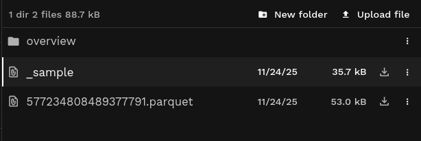
Overview file (/overview/hex7.parquet) — example rows (hex ID + aggregated value):

hex	data_avg
872830828ffffff	12.4
87283082effffff	8.2
87283082dffffff	15.1
87283082bffffff	3.7
872830829ffffff	22.0

Open in HyParquet to explore the full file.

---

Metrics

Choose metrics based on your raster data type:

Metric	Use Case	Output Columns
"cnt"	Categorical data (land use, crop types)	data, cnt, cnt_total
"avg"	Continuous averages (temperature, elevation, density)	data_avg
"sum"	Totals (population counts)	data_sum
"min", "max", "stddev"	Additional statistics	data_min, data_max, data_stddev

note

"cnt" cannot be combined with other metrics. Other metrics can be combined: metrics=["avg", "min", "max"]

Counting (categorical data)

For discrete/categorical rasters like land use, "cnt" counts occurrences per category:

CDL Example

@fused.udf
def udf(
    bounds: fused.types.Bounds = [-73.983, 40.763, -73.969, 40.773],
    res: int = None,
):
    # Cropland Data Layer ingested with "cnt" metric
    path = "s3://fused-asset/hex/cdls_v8/year=2024/"
    utils = fused.load("https://github.com/fusedio/udfs/tree/79f8203/community/joris/Read_H3_dataset")
    df = utils.read_h3_dataset(path, bounds, res=res)
    return df

                  hex  data  cnt  cnt_total
0  626740321835323391   122   12         14
1  626740321835323391   123    1         14
2  626740321835323391   121    1         14

Each H3 cell can have multiple rows (one per category).

Aggregating (continuous data)

For continuous rasters, aggregation produces one value per H3 cell:

DEM Example

@fused.udf
def udf(
    bounds: fused.types.Bounds = [-73.983, 40.763, -73.969, 40.773],
    res: int = None,
):
    path = "s3://fused-asset/hex/nyc_dem/"
    utils = fused.load("https://github.com/fusedio/udfs/tree/79f8203/community/joris/Read_H3_dataset")
    df = utils.read_h3_dataset(path, bounds, res=res)
    return df

                  hex   data_avg
0  617733122581069823  78.822576
1  617733122610954239  78.225562

---

Configuration

Data Resolution (res)

By default, resolution is inferred from raster pixel size. Override with res parameter.

See Resolution Guide for the full resolution table.

Partitioning (file_res, chunk_res)

Data is spatially partitioned using H3:

Parameter	Purpose	Default
file_res	Split into multiple files	Inferred (~100MB-1GB per file)
chunk_res	Row groups within files	Inferred (~1M rows per chunk)
max_rows_per_chunk	Alternative to chunk_res	-

Special case: file_res=-1 creates a single output file for smaller datasets.

Example

For data resolution 10: default file_res=0 (max 122 files globally) and chunk_res=3 (max 343 row groups per file, ~820k rows each assuming full coverage).

Overview Resolutions (overview_res)

Overviews are pre-aggregated files for fast zoomed-out views. Default: resolutions 3-7.

result_extract, result_partition = fused.h3.run_ingest_raster_to_h3(
    input_path,
    output_path,
    metrics=["avg"],
    overview_res=[7,6,5,4,3],  # Custom overview resolutions
)

Overview files are also chunked. Default chunk resolution is overview_res - 5. Override with overview_chunk_res or max_rows_per_chunk.

---

Multiple Files

Single file:

input_path = "s3://fused-asset/data/nyc_dem.tif"

Directory:

input_path = fused.api.list("s3://copernicus-dem-90m/")

Multiple paths:

input_path = [
    "s3://copernicus-dem-90m/.../file1.tif",
    "s3://copernicus-dem-90m/.../file2.tif",
]

Ingesting more than 20 files

When ingesting a single or up to 20 files, each file is processed in multiple chunks in the first "extract" step (number of chunks depending on target_chunk_size argument). But when processing more than 20 files, each file is processed as a single chunk by default (fetching the metadata of each input file to determine the chunking can take a lot of time if there are many input files). This might make the "extract" step require more memory. You can still override this default by specifying a specific target_chunk_size value.

info

Ingestion works with any hosted raster data - your files don't need to be on Fused's S3.

---

Execution Control

The ingestion runs these steps in parallel via .map():

1. extract: Assign pixel values to H3 cells
2. partition: Combine chunks per file, create metadata
3. overview: Create aggregated overview files

Override execution with:

• engine: Specify execution engine (e.g., "small", "medium", "c2-standard-4"). Use extract_engine, partition_engine and overview_engine to specify the execution engine for only a single step.
• max_workers and worker_concurrency: Control parallelism

Running on GCP

@fused.udf(engine="c2-standard-4")  # Orchestrator
def udf():
    result_extract, result_partition = fused.h3.run_ingest_raster_to_h3(
        input_path,
        output_path,
        metrics=["avg"],
        engine="c2-standard-60",  # Compute workers
    )

Planning the ingestion

Before running a full ingestion, you can estimate how large the output dataset will be and how much memory each pipeline step (extract, partition, overview) is likely to need. That helps you confirm the dataset is not unexpectedely huge and pick one of the engines required to run the ingestion.

The community UDF ingest_raster_to_h3_planning prints an estimate of the output size and per-step memory requirements. Pass the same keyword arguments you would pass to run_ingest_raster_to_h3 for the real ingestion (except output_path and keywords controlling the execution/engine):

@fused.udf(cache_max_age=0)
def udf():
    input_path = "s3://fused-asset/data/nyc_dem.tif"

    planner = fused.load("https://github.com/fusedio/udfs/tree/5b410e6/community/max/ingest_raster_to_h3_planning/")
    plan = planner(
        # pass the same arguments you would pass to the actual ingestion
        input_path,
        metrics=["avg"],
    )
    return plan

The UDF prints a breakdown of inferred or explicit resolutions, expected numbers of output files, row groups, and rows per file, plus per-step job counts and conservative memory estimates with suggested instance sizes when the workload is too heavy for a small realtime run.

If the output suggests to use a specific instance (e.g. "Consider using an 'r5.2xlarge' instance") for a certain step, you can either still use the default settings (which will first run on realtime, and then retry on a 'large' instance), or either specify the recommended instance specifically with e.g. partition_engine='r5.2xlarge'.

More than 20 input files

If you point at more than twenty source files, the planner will use only the first twenty file to estimate the extent of the dataset. Pass bounds (minx, miny, maxx, maxy) if the full extent matters.

---

Reading Ingested Data

Use read_h3_dataset to automatically select data vs overview files based on viewport:

@fused.udf
def udf(
    bounds: fused.types.Bounds = [-74.556, 40.400, -73.374, 41.029],
    res: int = None,
):
    path = "s3://fused-users/fused/joris/nyc_dem_h3/"
    utils = fused.load("https://github.com/fusedio/udfs/tree/dd40354/community/joris/Read_H3_dataset/")
    df = utils.read_h3_dataset(path, bounds, res=res)
    return df

Visualizing Ingested Data

Standalone map code

@fused.udf
def udf(
    bounds: fused.types.Bounds = [-74.556, 40.400, -73.374, 41.029],
    res: int = 9,
):
    path = "s3://fused-users/fused/joris/nyc_dem_h3/"
    utils = fused.load("https://github.com/fusedio/udfs/tree/dd40354/community/joris/Read_H3_dataset/")
    df = utils.read_h3_dataset(path, bounds, res=res)

    map_utils = fused.load("https://github.com/fusedio/udfs/tree/dd40354/community/milind/map_utils")
    config = {
        "hexLayer": {
            "@@type": "H3HexagonLayer",
            "filled": True,
            "pickable": True,
            "extruded": False,
            "opacity": 0.25,
            "getHexagon": "@@=properties.hex",
            "getFillColor": {
                "@@function": "colorContinuous",
                "attr": "data_avg",
                "domain": [0, 400],
                "steps": 20,
                "colors": "BrwnYl"
            }
        }
    }
    return map_utils.deckgl_hex(df, config=config)

For more on standalone maps, see Standalone Maps. For Workbench styling, see H3 Visualization.

---

Vector to H3

For vector data, use .map() to parallelize hexagonification:

Limits

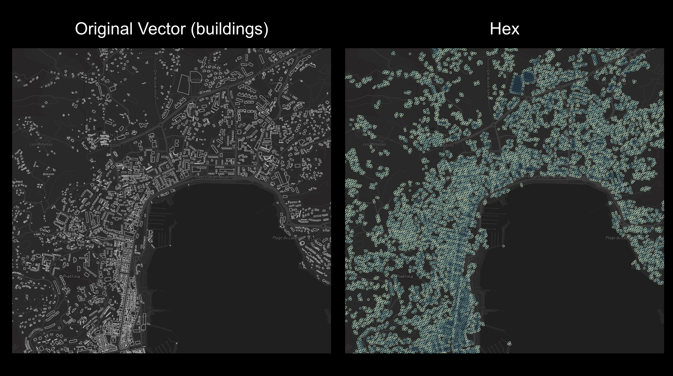
This method is for datasets < 100k vectors. Run in Single (viewport) mode, not Tiled.

@fused.udf
def udf(
    bounds: fused.types.Bounds = [8.4452104984018,41.76046948393174,8.903258920921276,42.053137175457145]
):
    common = fused.load("https://github.com/fusedio/udfs/tree/208c30d/public/common/")
    res = common.bounds_to_res(bounds, offset=0)
    res = max(9, res)
     
    gdf = get_data()

    if gdf.shape[0] > 100_000:
        print("Dataset too large. Contact info@fused.io for scaling.")
        return

    vector_chunks = common.split_gdf(gdf[["geometry"]], n=32, return_type="file")
    pool = hexagonify_udf.map(vector_chunks, res=res, engine="remote")
    df = pool.df().reset_index(drop=True)
    df = df.groupby('hex').sum(['cnt','area']).sort_values('hex').reset_index()[['hex', 'cnt', 'area']]
    df['area'] = df['area'].astype(int)

    return df 


@fused.udf
def hexagonify_udf(geometry, res: int = 12):
    common = fused.load("https://github.com/fusedio/udfs/tree/208c30d/public/common/")
    gdf = common.to_gdf(geometry)
    gdf = common.gdf_to_hex(gdf[['geometry']], res=15)
    con = common.duckdb_connect()
    df = con.execute(
        """
        SELECT h3_cell_to_parent(hex, ?) AS hex, 
               COUNT(1) AS cnt, 
               SUM(h3_cell_area(hex, 'm^2')) AS area
        FROM gdf
        GROUP BY 1
        ORDER BY 1
        """,
        [res],
    ).df()
    return df


@fused.cache
def get_data():
    gdf = fused.get_chunk_from_table(
        "s3://us-west-2.opendata.source.coop/fused/overture/2025-12-17-0/theme=buildings/type=building/part=3", 10, 0
    )
    return gdf

Open in Catalog →

Need help with larger datasets?

Reach out to our team at info@fused.io