Buffer: A Comprehensive Guide

Buffer analysis is a geospatial technique used to extract meaningful insights from location-based data. It helps determine which objects fall within a certain distance of Areas of Interest (AOIs) and account for possible inaccuracies in GPS data. This technique has various applications such as visit attribution and proximity analysis.

This tutorial shows a buffer analysis between a Point table and a LineString table to identify which vehicles are using specific roads. This approach can also be applied to other industry scenarios, such as determining which stores are within a certain distance of an area of interest (AOI) or which buildings are close to a body of water.

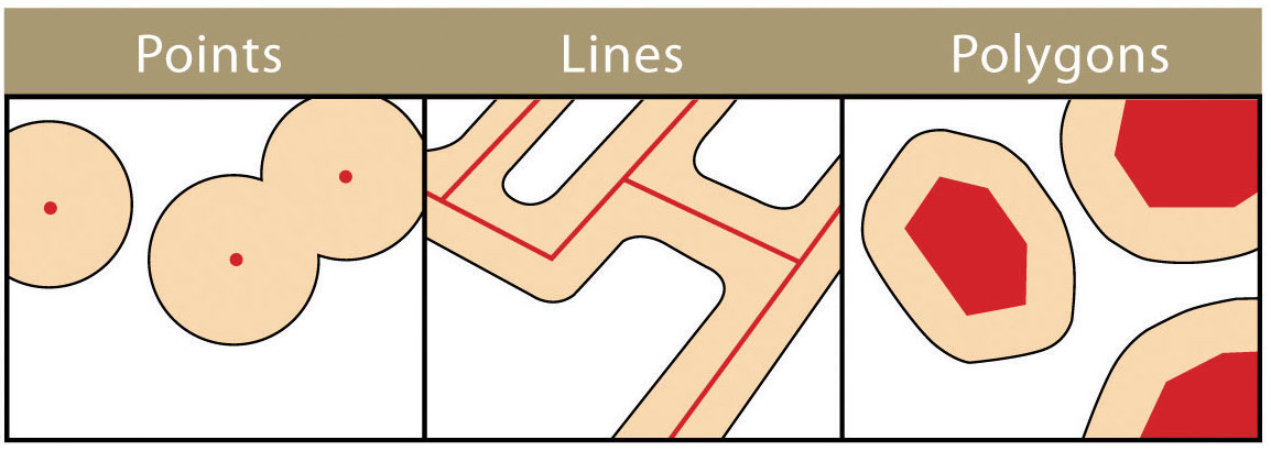
Visual representation of buffer around GeoPandas Point, LineString, and Polygon objects. Reference.

Applications

• Proximity analysis: Identify roads within a certain distance of specific landmarks
• Safety assessment: Pinpoint intersections prone to accidents
• Visit attribution: Determine visitors based on mobile GPS data to optimize store locations
• Site selection: Find buildings adjacent to parks
• Environmental monitoring: Identify watersheds within a certain distance of pollutant sources

Implementing buffer analysis

Implementation steps

To illustrate, we'll determine which vehicle GPS points fall within a buffer around a road. We can create a buffer zone around the road and check which GPS point fall within this area. Here's how to do this:

1. Represent road segments as LineStrings and vehicle GPS locations as Points
2. Create a buffer around a set of target roads
3. Call the within method to check which GPS points fall within the buffer

Example UDF

@fused.udf
def udf(n_points: int=1000, buffer: float=0.0025):
    import geopandas as gpd
    from shapely.geometry import Point, Polygon, LineString
    import random

    # Create LineString to represent a road
    linestring_columbus = LineString([[-122.4194,37.8065],[-122.4032,37.7954]])
    gdf_road = gpd.GeoDataFrame({'geometry': [linestring_columbus], 'name': ['Columbus Ave']})

    # Create Points to represent GPS pings
    minx, miny, maxx, maxy = gdf_road.total_bounds
    points = [Point(random.uniform(minx, maxx), random.uniform(miny, maxy)) for _ in range(n_points)]
    gdf_points = gpd.GeoDataFrame({'geometry': points})

    # Create a buffer around the road
    buffered_polygon = gdf_road.buffer(buffer)

    # Color the points that fall within the buffered polygon
    points_within = gdf_points[gdf_points.geometry.within(buffered_polygon.unary_union)]
    gdf_points = gdf_points.loc[points_within.index]

    return gdf_points

Conclusion

Buffer analysis is a powerful technique, but it's important to consider its limitations and potential complexities of the data. For example, in some scenarios you'll often find that buffers of different Areas of Interest (AOI) intersect which can lead to ambiguous situations where a single point falls within multiple buffers. The significance of a point falling within multiple buffers depends on the specifics of the use-case. For example:

• For road analysis, a car can't physically be on two roads simultaneously. In such cases, you'll need to employ additional techniques to resolve ambiguities, like determine speed or direction of travel.
• In other scenarios, like identifying "all buildings within 100m of any water body" overlapping buffers might not be problematic and could actually provide valuable insights.