Dark Vessel Detection
A complete example show casing how to use Fused to ingest data into a geo-partitioned, cloud friendly format, process images & vectors and use UDFs to produce an analysis
Requirements
- Access to Fused
- Access to a Jupyter Notebook
- Installing
fusedwith[all]dependencies (mainly to havepandas&geopandas):
pip install "fused[all]"
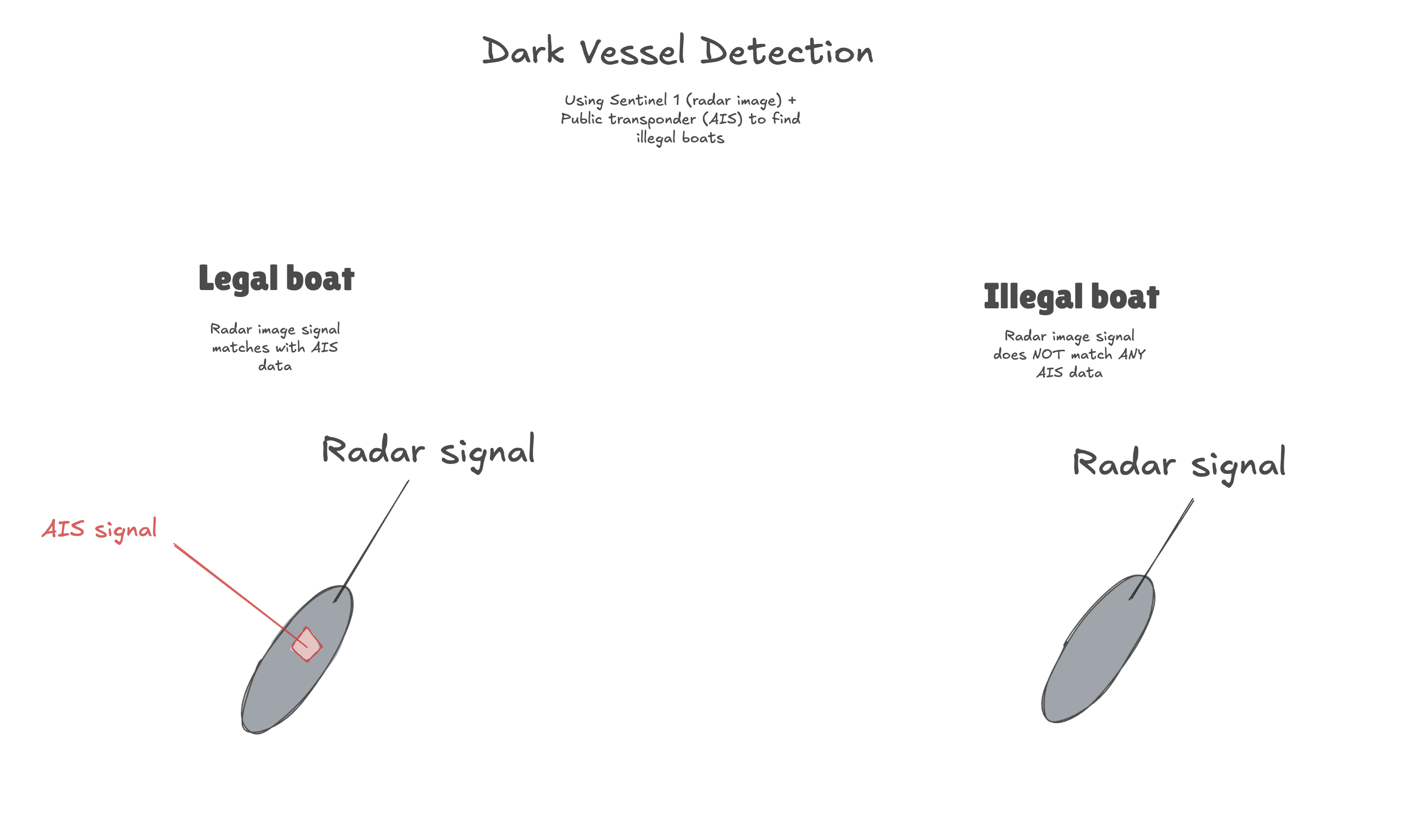
1. The problem: Detecting illegal boats
Monitoring what happens at sea isn't the easiest task. Shores are outfitted with radars and each ship has a transponder to publicly broadcast their location (using Automatic Identification System, AIS), but ships sometimes want to hide their location when taking part in illegal activities.
Global Fishing Watch has reported on "dark vessels" comparing Sentinel 1 radar images to public AIS data and matching the two to compare where boats report being versus where they actually are.
In this example, we're going to showcase a basic implementation of a similar analysis to identify potential dark vessels, all in Fused.
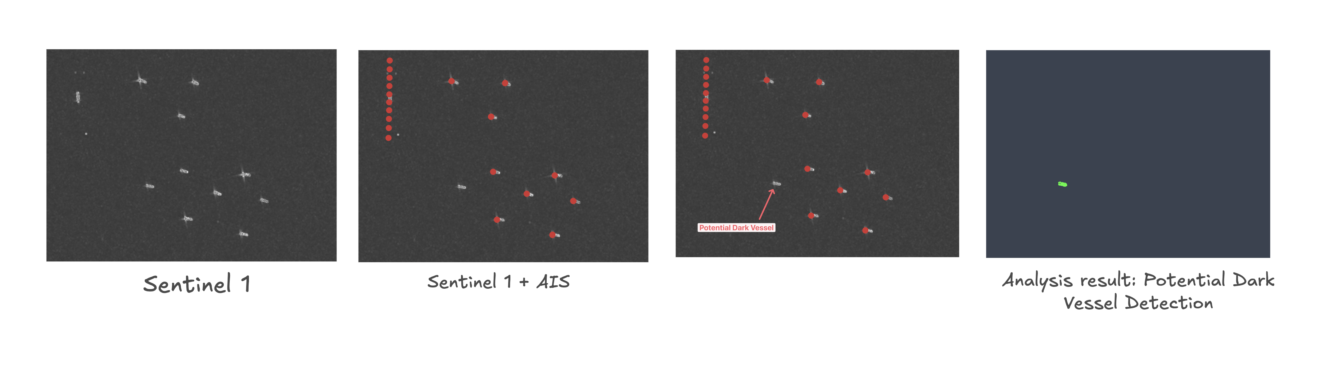
Here's the result of our analysis, running in real time in Fused:
Here are the steps we'll produce:
- Getting Sentinel 1 radar images over our Area of Interest and within our Time of Interest
- Run a simple algorithm to detect bright spots in radar images -> Return boats outline
- Fetch AIS data over the same Area & Time of Interest
- Merge the 2 datasets together
- Keep boats that appear in Sentinel 1 but not in AIS -> Those are our potential Dark Vessels.
This is crude analysis, mostly meant to demonstrate some of the major components of Fused, not to expose any dark vessels. The analysis has some major limitations and itself should be taken with a grain of salt.
That being said, we encourage you to use it as a starting point for your own work!
2. Data for our analysis
We will be using radar images and AIS data from free and open data sources for this study. Since we want to process and visualize this data, and iterate quickly, we want our datasets in a Cloud Native format. At the highest level and in practice this means that our data is:
- On a cloud storage (i.e. on S3 buckets)
- In a format that's fast to read and allows loading only small areas at a time (Cloud Optimized GeoTiff or GeoParquet)
The datasets we'll be accessing:
- Sentinel 1 radar images from Microsoft Planetary Computer Data Catalog
Specifics of the Sentinel 1 Dataset
For the nerds out there, we're using the Ground Range Detected product, not the Radiometrically Terrain Corrected because we're looking at boats in the middle of the ocean, so terrain shouldn't be any issue.
- This dataset is available as Cloud Optimized GeoTiff through a STAC Catalog, meaning we can directly use this data as is.
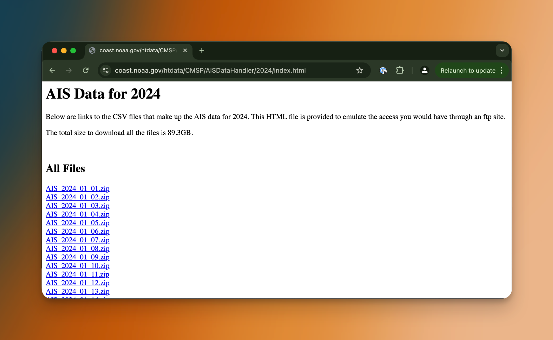
- AIS data from the NOAA Digital Coast. We have data all around the continental US per day as individual
.zipfiles- This dataset is not in a cloud native format. If we were to use this directly, every time we were to make a change to our analysis or look at a new area we'd have to find the correct
.zipfile, decompress it, read the entire AIS data for any given day then query only around our area of interest. This is possible, but brings out iteration speed from seconds to minutes.
- This dataset is not in a cloud native format. If we were to use this directly, every time we were to make a change to our analysis or look at a new area we'd have to find the correct
3. Ingesting AIS data
Since our AIS dataset is not in a geo-partitioned, cloud native format, our first step is to ingest it into a tiled format and put it on a cloud bucket. Thankfully we can do all of this in Fused. This will give us our 2014 AIS data on cloud storage in a GeoParquet format, allowing us to read data from small portions at a time.
To get this done we'll:
- Get a location to store our partitioned AIS data on (this can be any AWS S3 bucket, we'll use one managed by Fused to make this simpler)
- Write a simple UDF to unzip each AIS data over a given date range, read it and save it as a parquet file on S3
- Run this UDF over all of the 2024 AIS archive
- Ingest all of the monthly AIS
.parquetfiles into geo-partitioned files to speed up their read time over small areas
3.1 - Deciding on where to store out partitioned data
We first need to unzip & read our AIS data before ingesting in as a geo-partitioned cloud native format. One simple way to do this is to write a UDF that reads a zip file and saves it as .parquet file on a mounted disk.
AIS datapoint from NOAA's platform are available per day but we'll aggregate them per month to make it simpler to manage. We can run all of the code in this section in a notebook locally, since we don't need to visualize any data.
Fused UDFs by default run on serverless instances, so their local storage changes at every run. To keep data persistent across runs we use shared mounted storage across all the instances of your team
fused.file_path() returns the mount path of any file we'd like to create. When run locally, it returns the local /tmp/fused/ directory on your machine.
If this function is called inside a UDF, and that UDF is run on Fused servers, the returned path will be of the shared mounted storage /mount/. Specifying engine='local' runs the UDF on your local machine.
- Local
- In a UDF
- In a UDF run locally
import fused

datestr='2024_09_01'
path=fused.file_path(f'/AIS/{datestr[:7]}')
print(path)

>>> /tmp/fused/AIS/2024_09
If you run this code in the Fused Workbench or locally with fused.run() with default parameters, you'll see the /mount/ directory.
@fused.udf
def see_file_path():
    datestr='2024_09_01'
    path=fused.file_path(f'/AIS/{datestr[:7]}')
    print(path)
    return

fused.run(see_file_path)

>>> /mount/AIS/2024_09
You can see this directory in the File Explorer in Workbench.
@fused.udf
def see_file_path():
    datestr='2024_09_01'
    path=fused.file_path(f'/AIS/{datestr[:7]}')
    print(path)
    return

fused.run(see_file_path, engine='local')

>>> /tmp/AIS/2024_09
3.2 - Writing a UDF to open each AIS dataset
The rest of the logic is write a UDF to open each file, read it as a CSV and write it to parquet.
@fused.udf()
def read_ais_from_noaa_udf(datestr:str='2023_03_29', overwrite:bool=False):
    import os
    import requests
    import io
    import zipfile
    import pandas as pd
    import s3fs

    # This is the specific URL where daily AIS data is available
    url=f'https://coast.noaa.gov/htdata/CMSP/AISDataHandler/{datestr[:4]}/AIS_{datestr}.zip'

    # This is our local mount file path
    path=fused.file_path(f'/AIS/{datestr[:7]}/')
    daily_ais_parquet = f'{path}/{datestr[-2:]}.parquet'

    # Skipping any existing files
    if os.path.exists(daily_ais_parquet) and not overwrite:
        print(f'{daily_ais_parquet} exist')
        return pd.DataFrame({'status':['exist']})

    # Download ZIP file to mounted disk
    r=requests.get(url)
    if r.status_code == 200:
        with zipfile.ZipFile(io.BytesIO(r.content), 'r') as z:
            with z.open(f'AIS_{datestr}.csv') as f:
                df = pd.read_csv(f)
                # MMSI is the unique identifier of each boat. This is a simple clean up for demonstration
                df['MMSI'] = df['MMSI'].astype(str)
                df.to_parquet(daily_ais_parquet)
                print(f"Saved {daily_ais_parquet}")
        return pd.DataFrame({'status':['Done'], "file_path": [daily_ais_parquet]})
    else:
        return pd.DataFrame({'status':[f'read_error_{r.status_code}']})
We can run this UDF a single time to make sure it works:
single_ais_month = fused.run(read_ais_from_noaa_udf, datestr="2024_09_01")

>>> Saved /mnt/cache/AIS/2024_09/01.parquet
To recap what we've done so far:
- Build a UDF that takes a date, fetches a
.zipfile from NOAA's AISDataHandler portal and saves it to our UDFs' mount (so other UDFs can access it) - Run this UDF 1 time for a specific date
3.3 - Run this UDF over a month of AIS data
Next step: Run this for a whole period!
Since each UDF takes a few seconds to run per date, we're going to use fused.submit() to call a large numbers of UDFs all at once that will each run over a single date.
With a bit of Python gymnastics we can create a DataFrame of all the dates we'd like to process. Preparing to get all of September 2024 would look like this:
import pandas as pd
date_ranges = pd.DataFrame({
    'datestr': [str(i)[:10].replace('-','_') for i in pd.date_range('2024-09','2024-10')[:-1]]
})
print(f"{date_ranges.shape=}")
print(date_ranges.head())

>>> date_ranges.shape=(30, 1)
      datestr
0  2024_09_01
1  2024_09_02
2  2024_09_03
3  2024_09_04
4  2024_09_05
fused.submit() requires inputs as a list or DataFrame, in which case columns should have the argument names that our UDF expects, in this case datestr. We also recommend you always do a first run with debug_mode=True to test your submit job:
fused.submit(
    read_ais_from_noaa_udf,
    date_ranges,
    debug_mode=True
)

>>> Saved /mnt/cache/tmp/AIS/2024_09/01.parquet
  |status  | file_path
-------------------------------------------------
0 |Done    | /mnt/cache/tmp/AIS/2024_09/01.parquet
debug_mode=True runs the 1st value inside date_ranges with fused.run(). This allows you to make sure your UDF + arg_list combo is working properly.
Now that we've seen our UDF is working we can run all 30 jobs in parallel by removing debug_mode=True:
fused.submit(read_ais_from_noaa_udf, date_ranges)
We've now unzipped, opened & saved 30 days of data!
fused.submit() has more parameters you can control allowing you to change the number of max_workers, engine or the retry policies. Also take a look at the technical docs for more details.
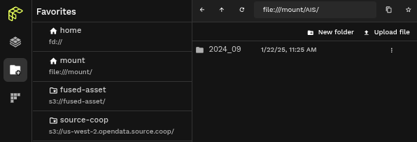
One handy way to make sure our data is in the right place is to check it in the Workbench File Explorer. In the search bar type: file:///mount/AIS/2024_09/:
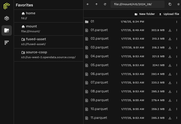
You'll see all our daily files! Notice how each file is a few 100 Mb. These files are still big individual files, i.e. would take a little while to read.
3.4 - Ingest 1 month of AIS data into a geo-partitioned format
These individual parquet files are now store on our mount disk. We could save them directly onto cloud storage but before that we can geo-partition them to make them even faster to read. This will make us reduce the time it takes to access our data from minutes to seconds. Fused provides a simple way to do this with the ingestion process.
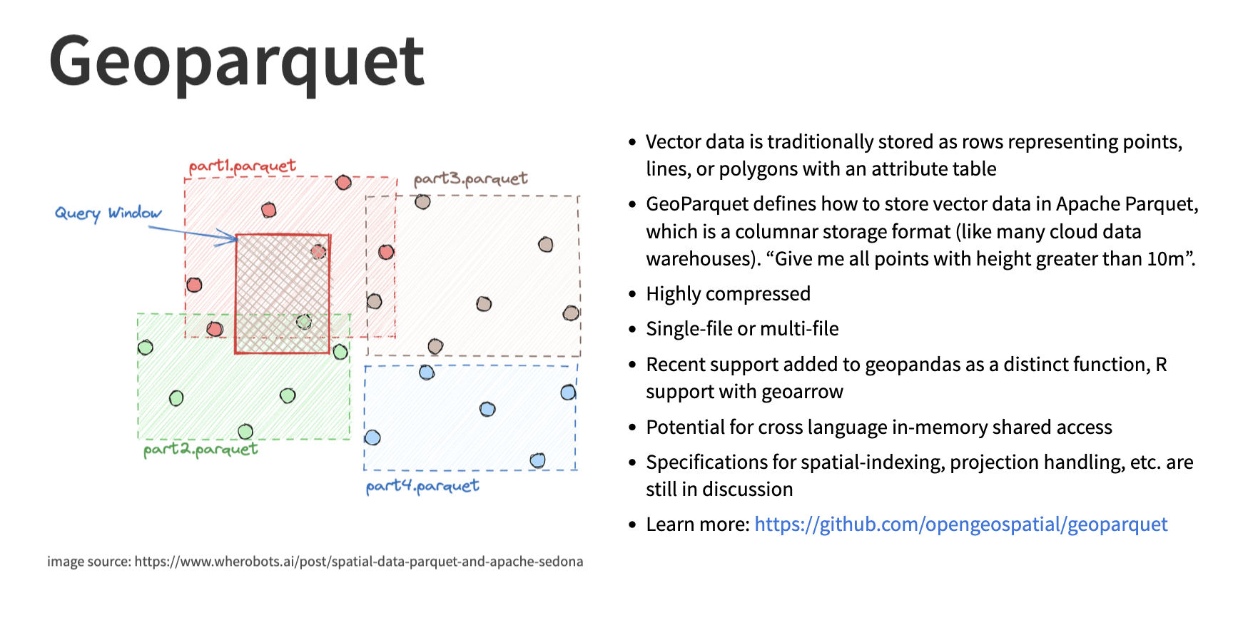
Image credit from the Cloud Native Geo slideshow
To do this we need a few things:
- Our input dataset: in this case our month of AIS data.
- A target cloud bucket: We're going to create a bucket to store our month of geo-partitioned AIS data in parquet files
- A target number of chunks to partition our data in. For now we're going to keep it at 500
- Latitude / Longitude columns to determine the location of each point
ais_daily_parquets = [f'file:///mnt/cache/AIS/{day[:-3]}/{day[-2:]}.parquet' for day in range_of_ais_dates]

job = fused.ingest(
    ais_daily_parquets,
    's3://fused-users/fused/demo_user/AIS_2024_ingester/prod_2024_09',
    target_num_chunks=500,
    lonlat_cols=('LON','LAT')
)
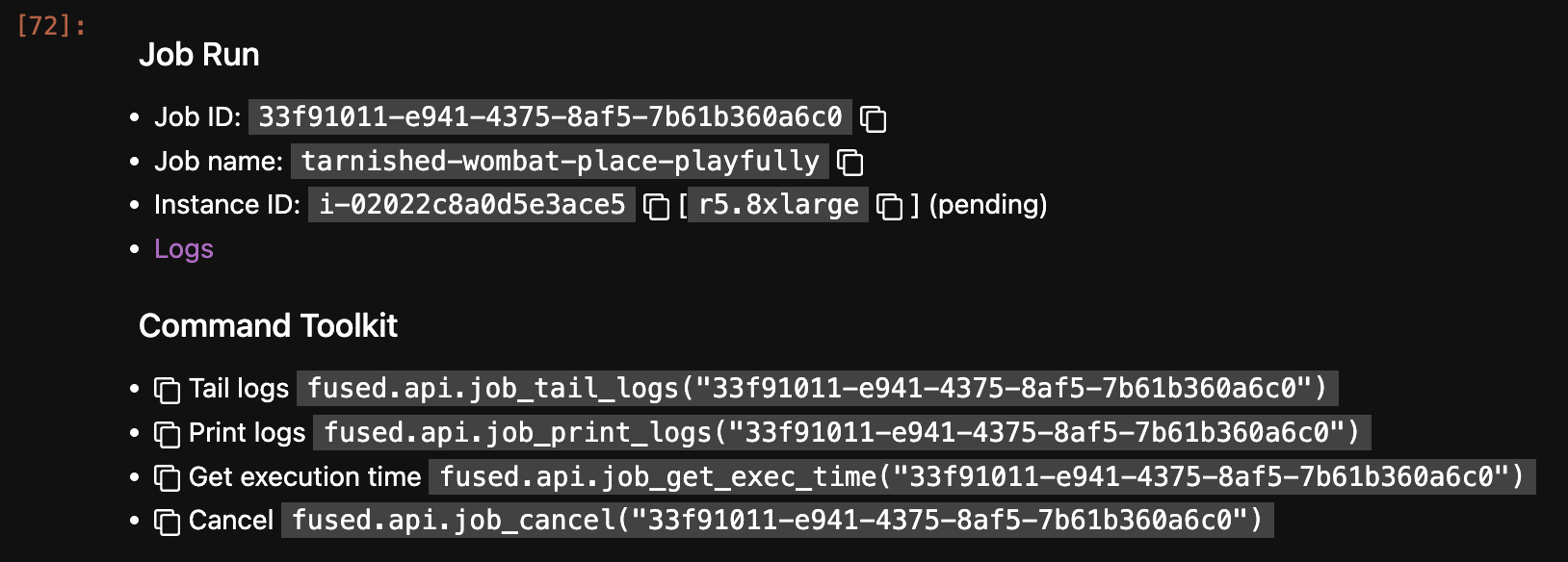
We'll send this job to a large instance using job.run_remote() as we latency doesn't matter much (we can wait a few extra seconds) and we'd rather have a larger machine & a larger storage:
job.run_remote(
    instance_type='r5.8xlarge', # We want why big beefy machine to do the partitioning in parallel, so large amounts of CPUs
    disk_size_gb=999 # Set a large amount of disk because this job will open each output parquet file to calculate centroid
)
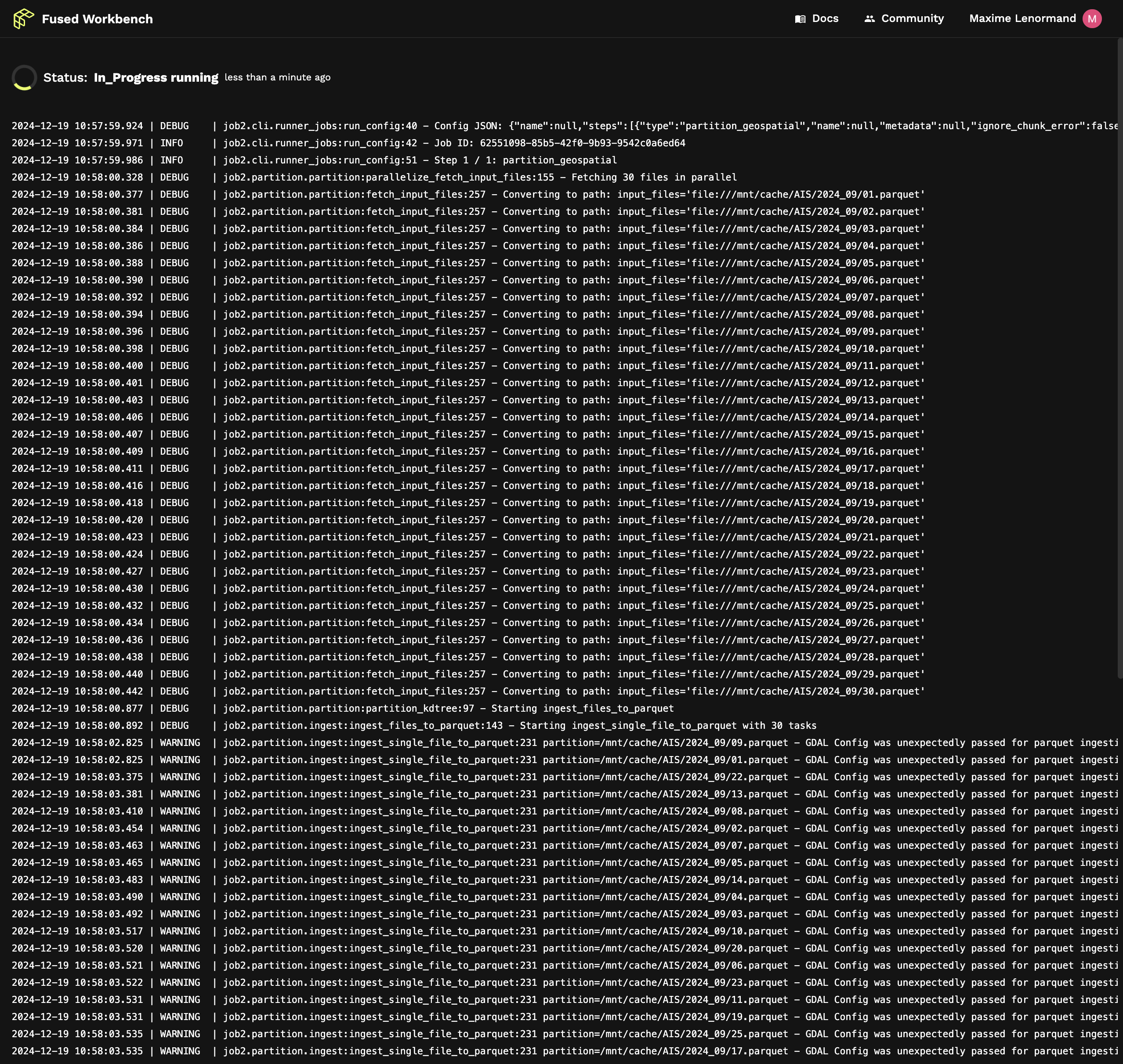
Running this in a notebook gives us a link to logs so we can follow the progress of the job on the offline machine:
Following the link shows us the live logs of what our job is doing:
We can once again check that our geo-partitioned images are available using File Explorer. This time because our files are a lot faster to read we can even see the preview in the map view:
Our AIS data is ready to be use for the entire month of September 2024. To narrow down our search, we now need to get a Sentinel 1 image. Since these images are taken every 6 to 12 days depending on the region, we'll find a Sentinel 1 image and then narrow our AIS data to just a few minutes before and after the acquisition time of the Sentinel 1 image.
4. Retrieving Sentinel 1 images
Sentinel 1 images are free & open, so thankfully for us others have already done the work of turning the archive into cloud native formats (and continue to maintain the ingestion as new data comes in).
We're going to use the Microsoft Planetary Computer Sentinel-1 Ground Range Detected dataset, because it offers:
- Access through a STAC Catalog helping us only get the data we need and nothing else
- Images are in Cloud Optimized Geotiff giving us tiled images that load even faster
- Examples of how to access the data so most of our work will be copy pasta
Most of the following section was written in Workbench's UDF Builder rather than in Jupyter Notebooks.
We'll have the code in code blocks, you can run these anywhere but as we're looking at images, it's helpful to have UDF Builders' live map updated as you write your code.
Let's start with a basic UDF just returning our area of interest:
@fused.udf
def udf(
    bounds: fused.types.Bounds,
):
    utils = fused.load("https://github.com/fusedio/udfs/tree/e1fefb7/public/common/").utils
    # Convert bounds to GeoDataFrame using Fused utility function
    bounds = utils.bounds_to_gdf(bounds)
    return bounds
The code above demonstrates a basic User-Defined Function (UDF) that utilizes Fused's utility functions. These utilities provide a some general functions for geospatial operations and transformations. You can also define your own utils in the utils section of the workbench.
The utility function bounds_to_gdf is mentioned above is defined as:
def bounds_to_gdf(bounds_list, crs=4326):
    import geopandas as gpd
    import shapely
    box = shapely.box(*bounds_list)
    return gpd.GeoDataFrame(geometry=[box], crs=crs)
This function converts a bounding box into a GeoDataFrame .
This UDF simply returns our Map viewport as a gpd.GeoDataFrame, this is a good starting point for our UDF returning Sentinel 1 images
While you can do this anywhere around the continental US (our AIS dataset covered shores around the US, so we want to limit ourselves there), if you want to follow along this is the area of interest we'll be using. You can overwrite this in the UDF directly:
@fused.udf
def udf(
    bounds: fused.types.Bounds,
):
    # Define our specific bounds
    specific_bounds = [-93.90425364, 29.61879782, -93.72767384, 29.7114987]
    utils = fused.load("https://github.com/fusedio/udfs/tree/e1fefb7/public/common/").utils
    bounds = utils.bounds_to_gdf(specific_bounds)
    return bounds
Following the Microsoft Planetary Computer examples for getting Sentinel-1 we can add a few of the imports we need and call the STAC catalog:
@fused.udf
def udf(
    bounds: fused.types.Bounds,
):
    import planetary_computer
    import pystac_client
    import geopandas as gpd
    import shapely
    # Define our specific bounds and convert to GeoDataFrame
    specific_bounds = [-93.90425364, 29.61879782, -93.72767384, 29.7114987]
    utils = fused.load("https://github.com/fusedio/udfs/tree/e1fefb7/public/common/").utils
    bounds = utils.bounds_to_gdf(specific_bounds)

    catalog = pystac_client.Client.open(
        "https://planetarycomputer.microsoft.com/api/stac/v1",
        # Details as to why we need to sign it are addressed here: https://planetarycomputer.microsoft.com/docs/quickstarts/reading-stac/#Searching
        modifier=planetary_computer.sign_inplace,
    )

    return bounds
We already have a bounding box, but let's narrow down our search to the first week of September:
@fused.udf
def udf(
    bounds: fused.types.Bounds,
):
    import planetary_computer
    import pystac_client
    import geopandas as gpd
    import shapely

    time_of_interest="2024-09-03/2024-09-04"
    specific_bounds = [-93.90425364, 29.61879782, -93.72767384, 29.7114987]
    utils = fused.load("https://github.com/fusedio/udfs/tree/e1fefb7/public/common/").utils
    bounds = utils.bounds_to_gdf(specific_bounds)

    catalog = pystac_client.Client.open(
        "https://planetarycomputer.microsoft.com/api/stac/v1",
        # Details as to why we need to sign it are addressed here: https://planetarycomputer.microsoft.com/docs/quickstarts/reading-stac/#Searching
        modifier=planetary_computer.sign_inplace,
    )

    items = catalog.search(
        collections=["sentinel-1-grd"],
        bbox=bounds.total_bounds,
        datetime=time_of_interest,
        query=None,
    ).item_collection()
    print(f"{len(items)=}")
    return bounds
This print statement should return something like:
Returned 15 Items
This will be the number of unique Sentinel 1 images covering our bounds and time_of_interest.
We can now use the odc package to load the first image & we'll use the VV polarisation from Sentinel 1 (VH could also work, and it would be good to iterate on this to visually assess which one would work best. We're keeping it simple for now, but feel free to test out both!).
We'll get an xarray.Dataset object back that we can simply open & return as a uint8 array:
@fused.udf
def udf(
    bounds: fused.types.Bounds,
):
    import odc.stac
    import planetary_computer
    import pystac_client
    import geopandas as gpd
    import shapely


    time_of_interest="2024-09-03/2024-09-04"
    bands = ["vv"]

    # Convert bounds to GeoDataFrame for STAC operations
    specific_bounds = [-93.90425364, 29.61879782, -93.72767384, 29.7114987]
    utils = fused.load("https://github.com/fusedio/udfs/tree/e1fefb7/public/common/").utils
    bounds = utils.bounds_to_gdf(specific_bounds)

    catalog = pystac_client.Client.open(
        "https://planetarycomputer.microsoft.com/api/stac/v1",
        # Details as to why we need to sign it are addressed here: https://planetarycomputer.microsoft.com/docs/quickstarts/reading-stac/#Searching
        modifier=planetary_computer.sign_inplace,
    )

    items = catalog.search(
        collections=["sentinel-1-grd"],
        bbox=bounds.total_bounds,
        datetime=time_of_interest,
        query=None,
    ).item_collection()
    print(f"{len(items)=}")

    ds = odc.stac.load(
        items,
        crs="EPSG:3857",
        bands=bands,
        resolution=10, # We want to use the native Sentinel 1 resolution which is 10m
        bbox=bounds.total_bounds,
    ).astype(float)

    da = ds[bands[0]].isel(time=0)
    image = da.values * 1.0
    return image.astype('uint8')
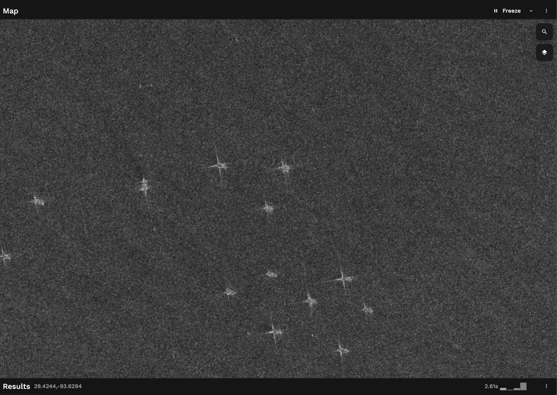
Which gives us a Sentinel 1 image over our area of interest:
We've simplified the process quite a bit here, you could also:
- Instead of loading
image.astype('uint8'), do a more controlled calibration and conversation to dB - Select a more specific image rather than the 1st one in our stack
- Use a different band or band combination
- Use Radiometrically Terrain Corrected images
4.1 Cleaning our Sentinel 1 UDF
Before adding any new functionality, we're going to clean our UDF up a bit more:
- Move some of the functionality into separate functions
- Adding common error catching (so our UDF doesn't fail if no Sentinel 1 images are found within our AOI + date range if it's too narrow)
- Add a cache decorator to code functions that retrieve data to speed up the UDF & reduce costs.
This will allow us to keep our UDF more readable (by abstracting code away) and more responsive. Cached functions store their result to disk, which makes a common query a lot more responsive and less expensive by using less compute
Here's our cleaned up UDF:
@fused.udf
def udf(
    bounds: fused.types.Bounds,
    bands: list=["vv"],
    resolution: int=10,
    time_of_interest: str="2024-09-03/2024-09-10",
):
    import pandas as pd
    da = get_data(bounds, time_of_interest, resolution, bands)

    image = da.values * 1.0
    return image.astype('uint8')

@fused.cache
def get_data(
    bounds: fused.types.Bounds,
    time_of_interest: str,
    resolution: int,
    bands: list,
    data_name: str="sentinel-1-grd"
):
    """
    Getting Sentinel Data from MPC
    Resolution is defined in meters as we're using EPSG:3857
    """
    import odc.stac
    import planetary_computer
    import pystac_client

    # Convert bounds to GeoDataFrame
    utils = fused.load("https://github.com/fusedio/udfs/tree/e1fefb7/public/common/").utils
    bounds = utils.bounds_to_gdf(bounds)

    if resolution < 10:
        print("Resolution shouldn't be lower than Sentinel 1 or 2 native resolution. Bumping to 10m")
        resolution = 10
        print(f"{resolution=}")

    catalog = pystac_client.Client.open(
            "https://planetarycomputer.microsoft.com/api/stac/v1",
            # Details as to why we need to sign it are addressed here: https://planetarycomputer.microsoft.com/docs/quickstarts/reading-stac/#Searching
            modifier=planetary_computer.sign_inplace,
        )

    items = catalog.search(
        collections=[data_name],
        bbox=bounds.total_bounds,
        datetime=time_of_interest,
        query=None,
    ).item_collection()

    if len(items) < 1:
        print(f'No items found. Please either zoom out or move to a different area')
    else:
        print(f"Returned {len(items)} Items")

        def odc_load(bbox,resolution, time_of_interest):
            ds = odc.stac.load(
                    items,
                    crs="EPSG:3857",
                    bands=bands,
                    resolution=resolution,
                    bbox=bounds.total_bounds,
                ).astype(float)
            return ds

        ds=odc_load(bounds,resolution, time_of_interest)
        da = ds[bands[0]].isel(time=0)
        return da
We can make this even simpler by moving the get_data function under the Utils tab in the Workbench UDF Editor:
- Editor
- Utils
@fused.udf
def udf(
    bounds: fused.types.Bounds,
    bands: list=["vv"],
    resolution: int=10,
    time_of_interest: str="2024-09-03/2024-09-10",
):
    from utils import get_data
    da = get_data(bounds, time_of_interest, resolution, bands)
    image = da.values * 1.0

    return image.astype('uint8')
@fused.cache
def get_data(
    bounds: fused.types.Bounds,
    time_of_interest: str,
    resolution: int,
    bands: list,
    data_name: str="sentinel-1-grd"
):
    """
    Getting Sentinel Data from MPC
    Resolution is defined in meters as we're using EPSG:3857
    """
    import odc.stac
    import planetary_computer
    import pystac_client
    import geopandas as gpd

    # Convert bounds to GeoDataFrame if needed
    if not isinstance(bounds, gpd.GeoDataFrame):
        utils = fused.load("https://github.com/fusedio/udfs/tree/e1fefb7/public/common/").utils
        bounds = utils.bounds_to_gdf(bounds)

    if resolution < 10:
        print("Resolution shouldn't be lower than Sentinel 1 or 2 native resolution. Bumping to 10m")
        resolution = 10
        print(f"{resolution=}")

    catalog = pystac_client.Client.open(
            "https://planetarycomputer.microsoft.com/api/stac/v1",
            # Details as to why we need to sign it are addressed here: https://planetarycomputer.microsoft.com/docs/quickstarts/reading-stac/#Searching
            modifier=planetary_computer.sign_inplace,
        )

    items = catalog.search(
        collections=[data_name],
        bbox=bounds.total_bounds,
        datetime=time_of_interest,
        query=None,
    ).item_collection()

    if len(items) < 1:
        print(f'No items found. Please either zoom out or move to a different area')
    else:
        print(f"Returned {len(items)} Items")

        def odc_load(bounds,resolution, time_of_interest):
            ds = odc.stac.load(
                    items,
                    crs="EPSG:3857",
                    bands=bands,
                    resolution=resolution,
                    bbox=bounds.total_bounds,
                ).astype(float)
            return ds

        ds=odc_load(bounds,resolution, time_of_interest)
        da = ds[bands[0]].isel(time=0)
        return da
5. Simple boat detection in Sentinel 1 radar images
Now that we have a Sentinel 1 image over a Area of Interest and time range, we can write a simple algorithm to return bounding boxes of the boats in the image. We're going to keep this very basic as we're optimizing for:
- Speed of execution: We want our boat detection algorithm to run in a few seconds at most while we're iterating. Especially at first when we're developing our pipeline, we want a fast feedback loop
- Simplicity: We're focused on demo-ing how to build an end-to-end pipeline with Fused in this example, not making the most thorough analysis possible. This should be a baseline for you to build upon!
Radar images over calm water tend to look black (as all the radar signal is reflect away from the sensor), while (mostly metallic) boats reflect back to the sensor appearing like bright spots in our image. A simple "boat detecting" algorithm is thus to do a 2D convolution and threshold the output to a certain pixel value:
- Editor
- Utils
@fused.udf
def udf(
    bounds: fused.types.Bounds,
    bands: list=["vv"],
    resolution: int=10,
    time_of_interest: str="2024-09-03/2024-09-10",
):
    import numpy as np
    from utils import get_data, quick_convolution

    da = get_data(bounds, time_of_interest, resolution, bands)
    image = da.values * 1.0

    convoled_image = quick_convolution(np.array(image), kernel_size=2)

    return convoled_image.astype('uint8')
@fused.cache
def get_data(
    bounds: fused.types.Bounds,
    time_of_interest: str,
    resolution: int,
    bands: list,
    data_name: str="sentinel-1-grd"
):
    """
    Getting Sentinel Data from MPC
    Resolution is defined in meters as we're using EPSG:3857
    """
    import odc.stac
    import planetary_computer
    import pystac_client


    # Convert bounds to GeoDataFrame
    utils = fused.load("https://github.com/fusedio/udfs/tree/e1fefb7/public/common/").utils
    bounds = utils.bounds_to_gdf(bounds)

    if resolution < 10:
        print("Resolution shouldn't be lower than Sentinel 1 or 2 native resolution. Bumping to 10m")
        resolution = 10
        print(f"{resolution=}")

    catalog = pystac_client.Client.open(
            "https://planetarycomputer.microsoft.com/api/stac/v1",
            # Details as to why we need to sign it are addressed here: https://planetarycomputer.microsoft.com/docs/quickstarts/reading-stac/#Searching
            modifier=planetary_computer.sign_inplace,
        )

    items = catalog.search(
        collections=[data_name],
        bbox=bounds.total_bounds,
        datetime=time_of_interest,
        query=None,
    ).item_collection()

    if len(items) < 1:
        print(f'No items found. Please either zoom out or move to a different area')
    else:
        print(f"Returned {len(items)} Items")

        def odc_load(bounds,resolution, time_of_interest):
            ds = odc.stac.load(
                    items,
                    crs="EPSG:3857",
                    bands=bands,
                    resolution=resolution,
                    bbox=bounds.total_bounds,
                ).astype(float)
            return ds

        ds=odc_load(bounds,resolution, time_of_interest)
        da = ds[bands[0]].isel(time=0)

        return da

def quick_convolution(input_array, kernel_size):
    import numpy as np
    shifted_images = []

    # Shifting the image in all combinations of directions (x, y) with padding
    for x in [-kernel_size, 0, kernel_size]:  # Shift left (kernel_size), no shift (0), right (kernel_size)
        for y in [-kernel_size, 0, kernel_size]:  # Shift up (kernel_size), no shift (0), down (kernel_size)
            shifted = pad_and_shift_image(input_array, x, y, pad_value=0, kernel_size=kernel_size)
            shifted_images.append(shifted)

    stacked_image = np.stack(shifted_images)
    return stacked_image.std(axis=0)

def pad_and_shift_image(img, x_shift, y_shift, pad_value=0, kernel_size: int = 3):
    import numpy as np
    """Pad and shift an image by x_shift and y_shift with specified pad_value."""

    padded_img = np.pad(img, pad_width=kernel_size, mode='constant', constant_values=pad_value)
    shifted_img = np.roll(np.roll(padded_img, y_shift, axis=0), x_shift, axis=1)

    return shifted_img[kernel_size:-kernel_size, kernel_size:-kernel_size]
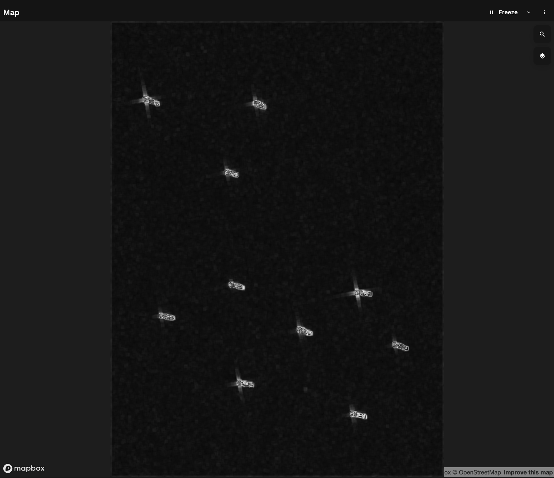
This returns a filtered image highlighting the brightest spots and reducing the natural speckle of the radar image
This is now relatively simple to vectorise (turn into a vector object, from image to polygons):
- Editor
- Utils
@fused.udf
def udf(
    bounds: fused.types.Bounds,
    bands: list=["vv"],
    resolution: int=10,
    time_of_interest: str="2024-09-03/2024-09-10",
):
    import geopandas as gpd
    import numpy as np
    from utils import get_data, quick_convolution, vectorise_raster
    utils = fused.load("https://github.com/fusedio/udfs/tree/e1fefb7/public/common/").utils
    bounds_gdf = utils.bounds_to_gdf(bounds)
    da = get_data(bounds, time_of_interest, resolution, bands)
    image = da.values * 1.0

    convoled_image = quick_convolution(np.array(image), kernel_size=2)

    gdf_predictions = vectorise_raster(
        raster=convoled_image.astype("uint8"),
        bounds=bounds_gdf,
        threshold=200 # Taking a high threshold in 0-255 range to keep only very bright spots
    )

    # Merging close polygons together into a single polygon so 1 polygon <-> 1 boat
    buffer_distance = 0.0001  # eyeballed a few meters in EPSG:4326 (degrees are annoying to work with ¯\_(ツ)_/¯)
    merged = gdf_predictions.geometry.buffer(buffer_distance).unary_union.buffer(
        -buffer_distance/2
    )
    merged_gdf = gpd.GeoDataFrame(geometry=[merged], crs=bounds.crs).explode()

    return merged_gdf
@fused.cache
def get_data(
    bounds: fused.types.Bounds,
    time_of_interest: str,
    resolution: int,
    bands: list,
    data_name: str="sentinel-1-grd"
):
    """
    Getting Sentinel Data from MPC
    Resolution is defined in meters as we're using EPSG:3857
    """
    import odc.stac
    import planetary_computer
    import pystac_client

    utils = fused.load("https://github.com/fusedio/udfs/tree/e1fefb7/public/common/").utils
    bounds = utils.bounds_to_gdf(bounds)
    if resolution < 10:
        print("Resolution shouldn't be lower than Sentinel 1 or 2 native resolution. Bumping to 10m")
        resolution = 10
        print(f"{resolution=}")

    catalog = pystac_client.Client.open(
            "https://planetarycomputer.microsoft.com/api/stac/v1",
            # Details as to why we need to sign it are addressed here: https://planetarycomputer.microsoft.com/docs/quickstarts/reading-stac/#Searching
            modifier=planetary_computer.sign_inplace,
        )
    items = catalog.search(
        collections=[data_name],
        bbox=bounds.total_bounds,
        datetime=time_of_interest,
        query=None,
    ).item_collection()

    if len(items) < 1:
        print(f'No items found. Please either zoom out or move to a different area')
    else:
        print(f"Returned {len(items)} Items")

        def odc_load(bounds,resolution, time_of_interest):
            ds = odc.stac.load(
                    items,
                    crs="EPSG:3857",
                    bands=bands,
                    resolution=resolution,
                    bbox=bounds.total_bounds,
                ).astype(float)
            return ds

        ds=odc_load(bounds,resolution, time_of_interest)
        da =  ds[bands[0]].isel(time=0)

        return da

def quick_convolution(input_array, kernel_size):
    import numpy as np
    shifted_images = []

    # Shifting the image in all combinations of directions (x, y) with padding
    for x in [-kernel_size, 0, kernel_size]: # Shift left (kernel_size), no shift (0), right (kernel_size)
        for y in [-kernel_size, 0, kernel_size]:  # Shift up (kernel_size), no shift (0), down (kernel_size)
            shifted = pad_and_shift_image(input_array, x, y, pad_value=0, kernel_size=kernel_size)
            shifted_images.append(shifted)

    stacked_image = np.stack(shifted_images)
    return stacked_image.std(axis=0)

def pad_and_shift_image(img, x_shift, y_shift, pad_value=0, kernel_size: int = 3):
    import numpy as np
    """Pad and shift an image by x_shift and y_shift with specified pad_value."""

    padded_img = np.pad(img, pad_width=kernel_size, mode='constant', constant_values=pad_value)
    shifted_img = np.roll(np.roll(padded_img, y_shift, axis=0), x_shift, axis=1)

    return shifted_img[kernel_size:-kernel_size, kernel_size:-kernel_size]

@fused.cache
def vectorise_raster(raster, bounds, threshold: float = 0.5):
    from rasterio import features
    import rasterio
    import geopandas as gpd
    import shapely
    import numpy as np

    transform = rasterio.transform.from_bounds(*bounds.total_bounds, raster.shape[1], raster.shape[0])

    shapes = features.shapes(
        source=raster.astype(np.uint8),
        mask = (raster > threshold).astype('uint8'),
        transform=transform
    )

    gdf = gpd.GeoDataFrame(
        geometry=[shapely.geometry.shape(shape) for shape, shape_value in shapes],
        crs=bounds.crs
    )
    return gdf
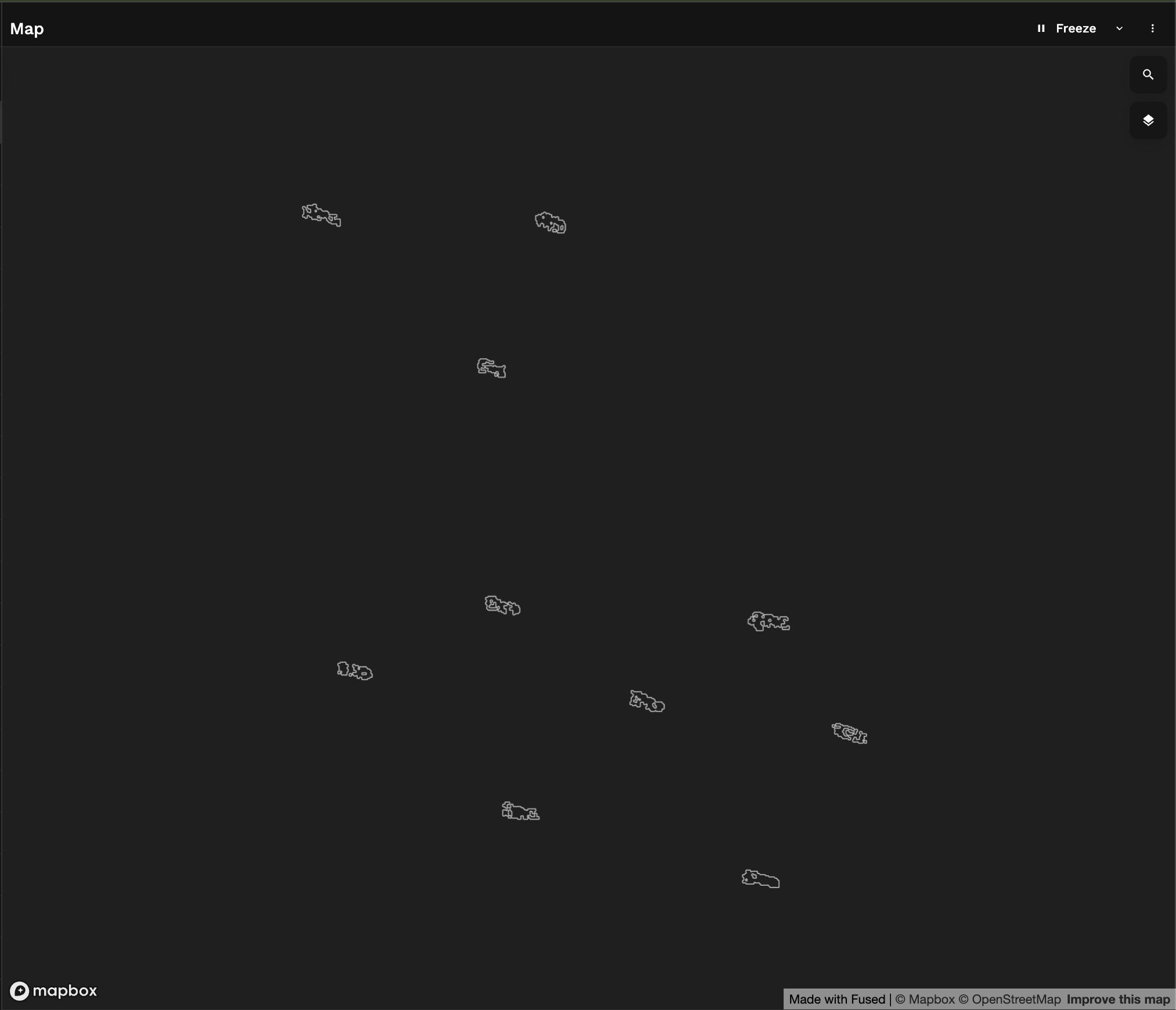
And that's how we have turned our Sentinel 1 image into a vector gpd.GeoDataFrame of bright objects:
6. Retrieving AIS data for our time of Interest
To get our AIS data, we now need to retrieve the exact moment our Sentinel 1 images were acquired. We can use this information to only keep AIS points within just a few minutes around that time.
- Editor
- Utils
def udf(
    bounds: fused.types.Bounds,
    bands: list=["vv"],
    resolution: int=10,
    time_of_interest: str="2024-09-03/2024-09-10",
):
    import geopandas as gpd
    import numpy as np
    from utils import get_data, quick_convolution, vectorise_raster

    utils = fused.load("https://github.com/fusedio/udfs/tree/e1fefb7/public/common/").utils
    bounds_gdf = utils.bounds_to_gdf(bounds)

    da = get_data(bounds, time_of_interest, resolution, bands)
    image = da.values * 1.0

    convoled_image = quick_convolution(np.array(image), kernel_size=2)

    gdf_predictions = vectorise_raster(
        raster=convoled_image.astype("uint8"),
        bounds=bounds_gdf,
        threshold=200 # Using higher threshold to make sure only bright spots are taken
    )

    # Merging close polygons together
    buffer_distance = 0.0001  # eyeballed value in EPSG:4326 so need to use degrees. I don't like degrees
    merged = gdf_predictions.geometry.buffer(buffer_distance).unary_union.buffer(
        -buffer_distance/2
    )
    merged_gdf = gpd.GeoDataFrame(geometry=[merged], crs=bounds.crs).explode()

    # Keeping metadata close by for merging with AIS data
    merged_gdf['S1_acquisition_time'] = da['time'].values

    return merged_gdf
@fused.cache
def get_data(
    bounds: fused.types.Bounds,
    time_of_interest: str,
    resolution: int,
    bands: list,
    data_name: str="sentinel-1-grd"
):
    """
    Getting Sentinel Data from MPC
    Resolution is defined in meters as we're using EPSG:3857
    """
    import odc.stac
    import planetary_computer
    import pystac_client

    utils = fused.load("https://github.com/fusedio/udfs/tree/e1fefb7/public/common/").utils
    bounds = utils.bounds_to_gdf(bounds)

    if resolution < 10:
        print("Resolution shouldn't be lower than Sentinel 1 or 2 native resolution. Bumping to 10m")
        resolution = 10
        print(f"{resolution=}")

    catalog = pystac_client.Client.open(
            "https://planetarycomputer.microsoft.com/api/stac/v1",
            # Details as to why we need to sign it are addressed here: https://planetarycomputer.microsoft.com/docs/quickstarts/reading-stac/#Searching
            modifier=planetary_computer.sign_inplace,
        )
    items = catalog.search(
        collections=[data_name],
        bbox=bounds.total_bounds,
        datetime=time_of_interest,
        query=None,
    ).item_collection()

    if len(items) < 1:
        print(f'No items found. Please either zoom out or move to a different area')
    else:
        print(f"Returned {len(items)} Items")

        def odc_load(bounds,resolution, time_of_interest):
            ds = odc.stac.load(
                    items,
                    crs="EPSG:3857",
                    bands=bands,
                    resolution=resolution,
                    bbox=bounds.total_bounds,
                ).astype(float)
            return ds

        ds=odc_load(bounds,resolution, time_of_interest)
        da =  ds[bands[0]].isel(time=0)

        return da

def quick_convolution(input_array, kernel_size):
    import numpy as np
    shifted_images = []

    # Shifting the image in all combinations of directions (x, y) with padding
    for x in [-kernel_size, 0, kernel_size]:  # Shift left (kernel_size), no shift (0), right (kernel_size)
        for y in [-kernel_size, 0, kernel_size]:  # Shift up (kernel_size), no shift (0), down (kernel_size)
            shifted = pad_and_shift_image(input_array, x, y, pad_value=0, kernel_size=kernel_size)
            shifted_images.append(shifted)

    stacked_image = np.stack(shifted_images)
    return stacked_image.std(axis=0)

def pad_and_shift_image(img, x_shift, y_shift, pad_value=0, kernel_size: int = 3):
    import numpy as np
    """Pad and shift an image by x_shift and y_shift with specified pad_value."""

    padded_img = np.pad(img, pad_width=kernel_size, mode='constant', constant_values=pad_value)
    shifted_img = np.roll(np.roll(padded_img, y_shift, axis=0), x_shift, axis=1)

    return shifted_img[kernel_size:-kernel_size, kernel_size:-kernel_size]

@fused.cache
def vectorise_raster(raster, bounds, threshold: float = 0.5):
    from rasterio import features
    import rasterio
    import geopandas as gpd
    import shapely
    import numpy as np

    transform = rasterio.transform.from_bounds(*bounds.total_bounds, raster.shape[1], raster.shape[0])

    shapes = features.shapes(
        source=raster.astype(np.uint8),
        mask = (raster > threshold).astype('uint8'),
        transform=transform
    )

    gdf = gpd.GeoDataFrame(
        geometry=[shapely.geometry.shape(shape) for shape, shape_value in shapes],
        crs=bounds.crs
    )
    return gdf
merged_gdf now returns a column called S1_acquisition_time with the time the Sentinel 1 image was taken.
If we save and call this UDF with a token we can call it from anywhere, from a Jupyter Notebook or from another UDF. Let's create a new UDF in Workbench:
# This is a new UDF
@fused.udf
def udf(
bounds: fused.types.Bounds=None,
time_of_interest: int="2024-09-03/2024-09-10",
):
import fused
@fused.cache()
def get_s1_detection(
time_of_interest=time_of_interest,
bounds=bounds):
return fused.run(
"fsh_673giUH9R6KqWFCOQtRfb3",
time_of_interest=time_of_interest,
bounds=bounds,
)
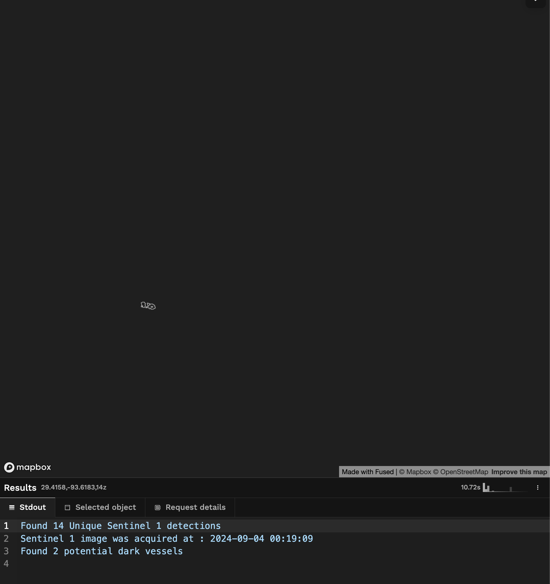
s1_detections = get_s1_detection()
print(f"Found {s1_detections.shape[0]} Unique Sentinel 1 detections")
# We want to keep AIS data only right around the time the S1 image was acquired
s1_acquisition_date = s1_detections['S1_acquisition_time'].values[0]
s1_acquisition_month = str(s1_acquisition_date.astype('datetime64[M]'))
s1_acquisition_month_day_hour_min = s1_acquisition_date.astype('datetime64[s]').astype(str).replace('T', ' ')
print(f"Sentinel 1 image was acquired at : {s1_acquisition_month_day_hour_min}")
return s1_detections
This prints out:
Found 16 Unique Sentinel 1 detections
Sentinel 1 image was acquired at : 2024-09-04 00:19:09
We can now create another UDF that will take this s1_acquisition_month_day_hour_min date + a bounding box in input and returns all the AIS points in that time + area.
We're going to leverage code from the community for this part, namely reading the AIS data from a geo-partitioned GeoParquet. Fused allows us to easily re-use any code we want and freeze it to a specific commit so it doesn't break our pipelines (read more about this here)
We can use this bit of code called table_to_tile which will either load the AIS data or the bounding box depending on our zoom level to keep our UDF fast & responsive.
You could write a GeoParquet reader from scratch or call a UDF that you have that already does this, you don't have to use this option. But we want to show you how you can re-use bits of code from others here.
@fused.udf
def udf(
    bounds: fused.types.Bounds = None,
    s1_acquisition_month_day_hour_min:str = '2024-09-04T00:19:09.175874',
    time_delta_in_hours: float = 0.1, # by default 6min (60min * 0.1)
    min_zoom_to_load_data: int = 14,
    ais_table_path: str = "s3://fused-users/fused/demo_user/AIS_2024_ingester/prod_2024_09", # This is the location where we had ingested our geo-partitioned AIS data
    ):
    """Reading AIS data from Fused partitioned AIS data from NOAA (data only available in US)"""
    import pandas as pd
    from datetime import datetime, timedelta

    # Load the utils module
    local_utils = fused.load("https://github.com/fusedio/udfs/tree/bb712a5/public/common/").utils
    zoom = local_utils.estimate_zoom(bounds)

    sentinel1_time = pd.to_datetime(s1_acquisition_month_day_hour_min)
    time_delta_in_hours = timedelta(hours=time_delta_in_hours)

    month_date = sentinel1_time.strftime('%Y_%m')
    monthly_ais_table = f"{ais_table_path}prod_{month_date}/"
    print(f"{monthly_ais_table=}")

    @fused.cache
    def getting_ais_from_s3(bounds, monthly_table):
        return local_utils.table_to_tile(
            bounds,
            table=monthly_ais_table,
            use_columns=None,
            min_zoom=min_zoom_to_load_data
        )

    ais_df = getting_ais_from_s3(bounds, monthly_ais_table)

    if ais_df.shape[0] == 0:
        print("No AIS data within this bounds & timeframe. Change bounds or timeframe")
        return ais_df

    if zoom > min_zoom_to_load_data:
        print(f"Zoom is {zoom=} | Only showing bounds")
        return ais_df

    print(f"{ais_df['BaseDateTime'].iloc[0]=}")
    ais_df['datetime'] = pd.to_datetime(ais_df['BaseDateTime'])
    mask = (ais_df['datetime'] >= sentinel1_time - time_delta_in_hours) & (ais_df['datetime'] <= sentinel1_time + time_delta_in_hours)
    filtered_ais_df = ais_df[mask]
    print(f'{filtered_ais_df.shape=}')
    return filtered_ais_df
In workbench UDF builder we can now see the output of both of our UDF:
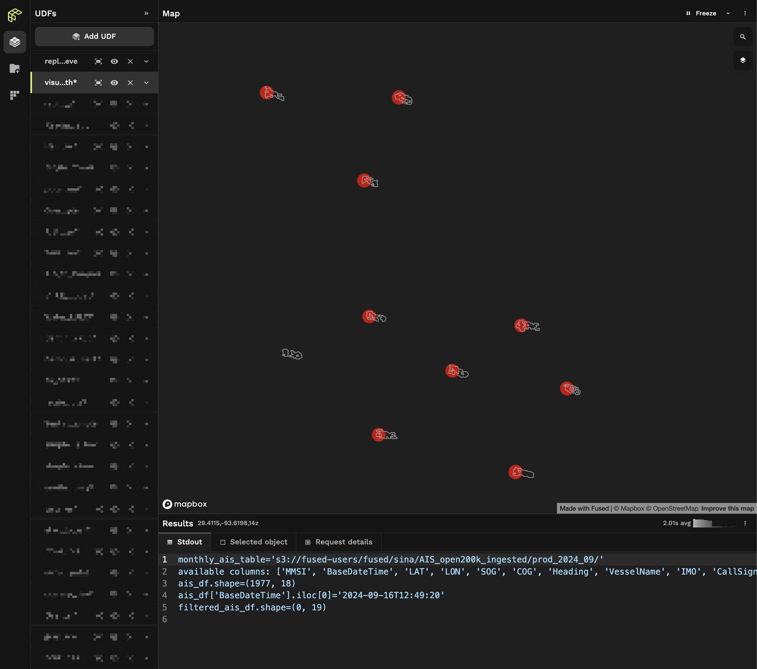
We can now see that 1 of these boats doesn't have an associated AIS point (in red).
You can change the styling of your layers in the Visualize tab to make them look like the screenshot above
Now all we need to do is merge these 2 datasets together and keep all the boats that don't match an AIS point.
7. Merging the 2 datasets together
We can expand the UDF we had started in section 6. to call our AIS UDF by passing a bounding box + s1_acquisition_month_day_hour_min.
We'll get the AIS data and join it with the Sentinel 1 detected boats by using geopandas sjoin_nearest to get the nearest distance of each boat to an AIS point.
Any point with the closest AIS point >100m from the Sentinel 1 boat will be considered a potentiel "dark vessel".
@fused.udf
def udf(
    bounds: fused.types.Bounds=None,
    time_of_interest: str="2024-09-03/2024-09-10",
    ais_search_distance_in_meters: int=10,
):
    import fused

    @fused.cache()
    def get_s1_detection(
        time_of_interest=time_of_interest,
        bounds=bounds):

        return fused.run(
            "fsh_673giUH9R6KqWFCOQtRfb3",
            time_of_interest=time_of_interest,
            bounds=bounds,
        )

    s1_detections = get_s1_detection()
    print(f"Found {s1_detections.shape[0]} Unique Sentinel 1 detections")

    # We want to keep AIS data only right around the time the S1 image was acquired
    s1_acquisition_date = s1_detections['S1_acquisition_time'].values[0]
    s1_acquisition_month = str(s1_acquisition_date.astype('datetime64[M]'))
    s1_acquisition_month_day_hour_min = s1_acquisition_date.astype('datetime64[s]').astype(str).replace('T', ' ')
    print(f"Sentinel 1 image was acquired at : {s1_acquisition_month_day_hour_min}")

    @fused.cache()
    def get_ais_from_s1_date(s1_acquisition_month_day_hour_min=s1_acquisition_month_day_hour_min, bounds=bounds):
        return fused.run("fsh_FI1FTq2CVK9sEiX0Uqakv", s1_acquisition_month_day_hour_min=s1_acquisition_month_day_hour_min, bounds=bounds)

    ais_gdf = get_ais_from_s1_date()

    # Making sure both have the same CRS
    s1_detections.set_crs(ais_gdf.crs, inplace=True)

    # Buffering AIS points to leverage spatial join
    ais_gdf['geometry'] = ais_gdf.geometry.buffer(0.005)

    joined = s1_detections.to_crs(s1_detections.estimate_utm_crs()).sjoin_nearest(
        ais_gdf.to_crs(s1_detections.estimate_utm_crs()),
        how="inner", # Using left, i.e. s1 as keys
        distance_col='distance_in_meters',
    )

    # Dark vessels will be unique S1 points that don't have an AIS point within 10m
    potential_dark_vessels = joined[joined['distance_in_meters'] > ais_search_distance_in_meters]
    print(f"Found {potential_dark_vessels.shape[0]} potential dark vessels")

    # back to EPSG:4326
    potential_dark_vessels.to_crs(s1_detections.crs, inplace=True)
    return potential_dark_vessels
And now we have a UDF that takes a time_of_interest and bounding box and returns potential dark vessel:
Limitations & Next steps
This is a simple analysis, that makes a lot of relatively naive assumptions (for ex: all bright spots in SAR are boats for example, which only works in open water and not near the shore or around solid structures like ocean wind mills or oil rigs). There's a lot of ways in which it could be improved but provides a good starting point.
This could be improved in a few ways:
- Masking out any shore or known areas with static infrastructure (to limit potential false positives around coastal wind mill farms)
Example of the Block Island Wind Farm in Rhode Island showing up as false positive "potential dark vessel": Wind mills appear as bright spots but don't have any AIS data associated to them
(bounds=[-71.08534386325134,41.06338103121641,-70.89011235861962,41.15718153299125] & s1_acquisition_month_day_hour_min = "2024-09-03T22:43:33")
- Using a more sophisticated algorithm to detect boats. The current algorithm is naive, doesn't return bounding boxes but rather general shapes.
- Return more information derived from AIS data: Sometimes boats go dark for a certain period of time only, making it possible to tie a boat that was dark for a certain time to a known ship when it does have it's AIS on.
- Running this over all the coast of the continental US and/or over a whole year. This would be closer to the Global Fishing Watch dark vessel detection project.
If you want to take this a bit further check out:
- Running UDFs at scale with
run_remote(). You could use this to run this pipeline over a larger area or over a much longer time series (or both!) to find out more potentiel dark vessels - More about Fused core concepts like chosing between running UDFs based on Tile or File