Analyzing traffic speeds from 100 billion drive records

Over the last few decades, it has become increasingly evident that passenger vehicles are by far the most dangerous way to travel. As a result, it has become more and more important to find an efficient and effective method to predict traffic risk. However, predicting traffic accidents and where they are likely to occur is a very complex problem, with large amounts of data being needed for most meaningful predictions.

At Pacific Spatial Solutions, we are currently trying to tackle this problem by training a machine learning model to predict road and intersection risk in Japan nationwide. As we are trying to predict traffic risk on a national level it is only natural that the data we use cover the same area.

The following UDF has been developed with data and support from MS&AD InterRisk Research & Consulting, Inc.

Challenges when working with big data

Generally, data processing and feature engineering are one of the most important steps of any ML pipeline, we are therefore working with Fused to help streamline and improve the costliest part of our data preparation stage.

The data in question is drive recorder data, in other words, data that cars send every other second to describe what condition the car was in at that point in time. For example, the speed the car was traveling at and if any of the internal warning lights were activated. With a fleet of thousands of cars sending this data every other second, the data grows extremely large very quickly. The dataset in question has hundreds of billions of rows. Working with data this large presents many unique challenges as even the simplest operations can take hours and cost thousands of dollars. Consequently, the process of finding the best way to utilize this type of data becomes a very time consuming and costly process.

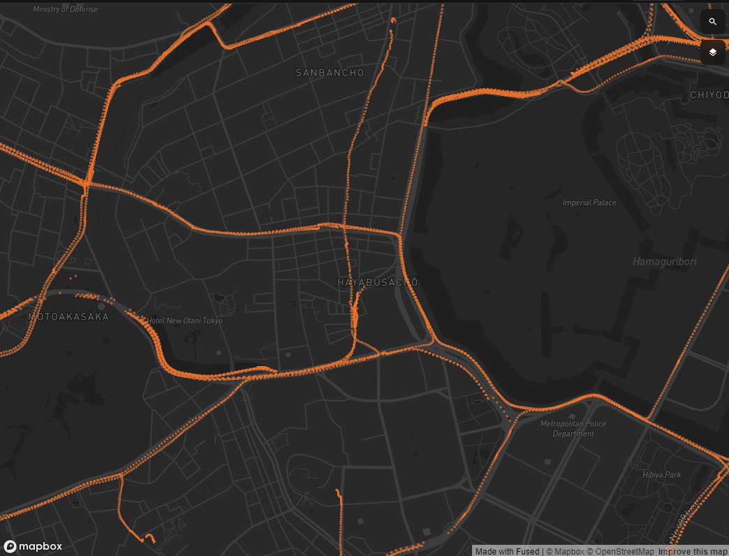
Drive recorder data points from a single day in a specific part of downtown Tokyo.

Moving to Fused

Specifically, what we are trying to achieve is to map the speed values from the drive recorder data points to their nearest road. Using a traditional “nearest neighbor” approach would not be feasible, as we would need to measure the distance between billions of points and thousands of roads. With our current cloud service provider we therefore had to rely on “clustering”, so that data points that are close location wise would be close in memory too. This definitely increases performance, but adds some randomness to the processing time and cost because depending on where the area of interest lies in memory, you might have to search through all of your data to find it. As a result, to keep cost and processing time reasonable, we had to limit the nearest neighbor search area using a very small buffer. This was the only way to make our analysis with a dataset of this magnitude feasible.

In Fused however, our spatial data uses a smart spatial partitioning system so that we know exactly where to look when attempting to spatially join our data. Furthermore, we can easily analyze and in real time visualize small chunks of the data and finetune our logic before scaling our implementation. This gives us a lot of freedom during development so that we can really hone in on the best possible solution to our problem.

This is very much in contrast to our cloud service provider, where we would need to move data around several times during development to visualize temporary results and do sanity checks. This made the development process very tedious and forced us into a simplified solution due to the limitations of the tool we were using.

Creating a scalable solution

Our solution is divided into two main steps the first being the preparation and ingestion of the road and drive recorder data, and the second being the UDF that analyzes the data after it has been prepared. We will be using the H3 spatial index to improve performance.

Ingestion

1. Ingest and spatially partition the point and road data directly from our data warehouse
2. Initialize DuckDB instance and add H3 index to our points and multiple H3 Kring indexes to the road data
3. Create metadata files to keep track of the geometry and H3 mapping

The reason why we add multiple Krings to the roads is that this will act like a hexagonized buffer. This will be much faster to search through as we will be doing number on number comparisons instead of geospatial distance measurements.

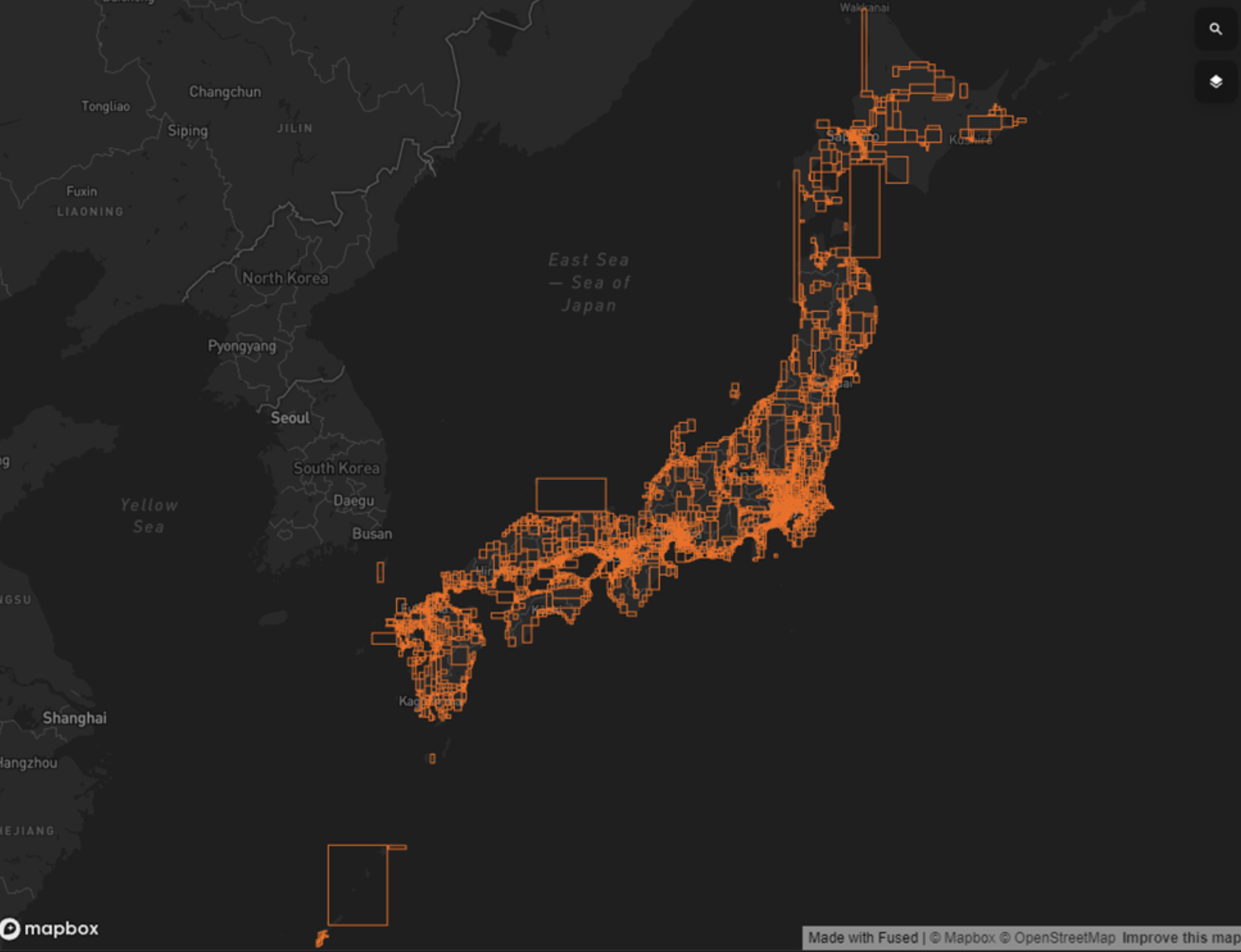
Nationwide drive recorder data points and their Fused spatial partitions.

UDF Design

1. Use bbox to load GPS points and roads in the viewport.
2. Structure DataFrames with the GPS points, road krings and road geometry.
3. For each point identify the road with the closest kring cell within a certain k distance, and map the speed to it.
4. Aggregate all of the speed values.

@fused.udf
def udf(
    bbox: fused.types.TileGDF=None,
    base_path: str = '...'
):
    from utils import df_to_gdf, list_s3, run_pool, get_GPS_road_data

    # Load ingested GPS and road data
    L = list_s3(f'{base_path}/GPS_hex/')
    df_GPS, df_road_hex, df_road_geom = get_GPS_road_data(bbox, L)

    # Nearest neighbor calculation
    df_final = df_GPS.merge(df_road_hex, on='hexk')
    df_final['distance'] = (df_final['k']+0.5)*k
    df_final['cnt'] = 1
    dfg = df_final.groupby('segment_id')[['cnt', 'speed', 'distance']].sum().reset_index()
    dfg['speed'] = dfg['speed']/dfg['cnt']
    dfg['distance'] = dfg['distance']/dfg['cnt']

    # Introduce geometry to roads
    df = df_road_geom.merge(dfg)
    df['width_metric'] = df['cnt']**0.5/5
    return df.sjoin(bbox[['geometry']])

We now have our result which is a DataFrame representing the road network within our bbox. All the roads have their respective aggregated speed, distance and metric values as well as how many points were used for the aggregation. This result can easily be enriched by bringing in more columns from the base data such as the timestamp. This would make it possible to create hourly speed pattern analysis or maybe even a time series visualization.

For demonstration purposes, the video above shows this UDF running on a fraction of the ingested dataset.

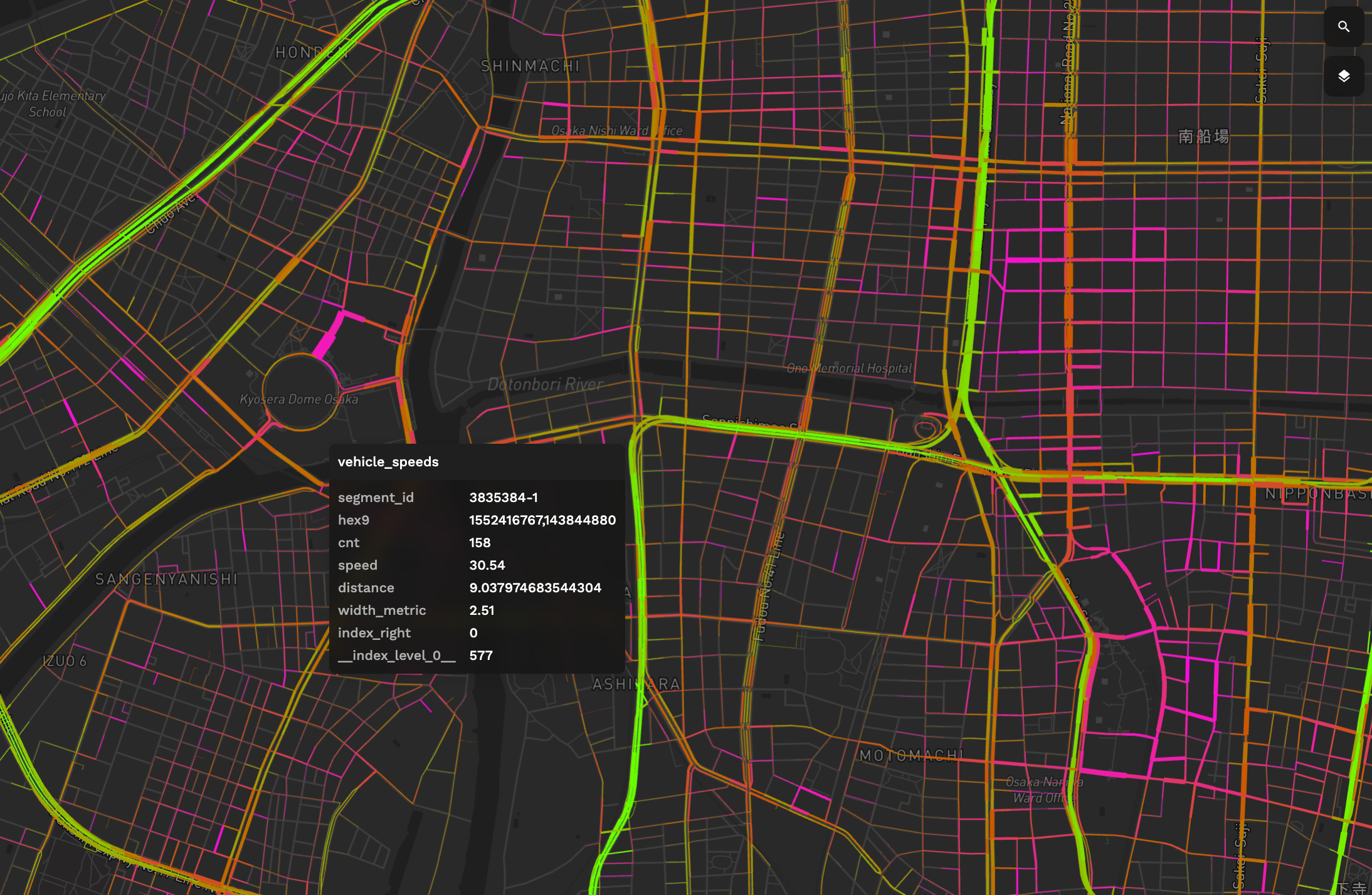
UDF result of Osaka Japan. Line width shows point density. Brighter yellow colors indicate high speed and darker purple colors low speed.

Conclusion

By leveraging the spatial partitioning that Fused does during ingestion and the flexibility of the h3 library, we have created a method to reliably map our drive recorder points to their nearest segment.

The natural next step will be to scale our analysis using multiple machines and run on all of our data. To achieve this, we would iterate over each of the chunks that fused produced when ingesting our road data, instead of the bbox. This will ensure that our calculations are only run once for each of our roads. The modification can be achieved fairly easily in Fused and we are very excited to see how well Fused will be able to perform in this case.